Most R&D teams don't start with a modeling problem. They start with a lab problem.
A formulation looks promising. A process tweak improves yield. Then progress stalls. You raise temperature and get a gain. You change concentration and performance slips. You bring temperature back down and suddenly the earlier conclusion no longer holds. The issue isn't that the science is unclear. It's that the variables are interacting, and one-factor-at-a-time testing can't show that cleanly.
That's where response surface modeling becomes practical, not academic. It gives teams a disciplined way to learn how multiple inputs move a response together, and it helps them spend experimental budget on the runs that sharpen decisions. In modern R&D, that matters even more because the same logic now underpins many AI-guided experiment planning systems. The classical method is still doing the heavy lifting. The software just makes it easier to use well.
Table of Contents
- Beyond Trial and Error Experimentation
- A map for a surface you can't see directly
- The three pieces that matter
Beyond Trial and Error Experimentation
A common pattern in materials and process development looks like this. A team adjusts resin content, then curing temperature, then mixing speed, hoping each isolated change will reveal the winning setting. Early on, that works well enough. Later, it stops working because the process no longer behaves like a set of independent knobs.
One-factor-at-a-time testing tends to hide the exact effects that matter most near an optimum. You can miss the point where temperature helps only up to a threshold. You can miss the point where pressure matters only when flow rate is in a certain range. You can also misread a factor entirely because its value depends on what the other factors are doing.
Practical rule: If your process response changes direction after a few “successful” tweaks, don't assume the chemistry became unpredictable. Assume the variables are interacting.
Response surface modeling is a better operating system for that situation. Instead of asking, “What happens if I change this one factor next?” it asks, “What shape does the response take across the region I care about?” That shift matters. It turns optimization from trial-and-error into a structured search.
In practice, teams use response surface modeling when they need to optimize multiple controllable factors against a measurable output such as yield, strength, uniformity, cure quality, or defect rate. The method is especially useful when experiments are expensive, pilot time is scarce, or simulation runs take too long to brute-force.
A strong RSM workflow usually changes behavior in three ways:
- It replaces random follow-up runs with an intentional experimental design.
- It exposes interactions that OFAT work often misses.
- It gives the team a predictive surface, not just a notebook full of disconnected observations.
That's why experienced R&D groups keep coming back to it. The method doesn't remove uncertainty. It helps you spend uncertainty wisely.
What Is Response Surface Modeling
Response surface modeling is easiest to understand as a search problem. You're trying to find the highest point on a surface you can't see directly. Each experiment gives you one measured location. The model turns those scattered measurements into a usable map.
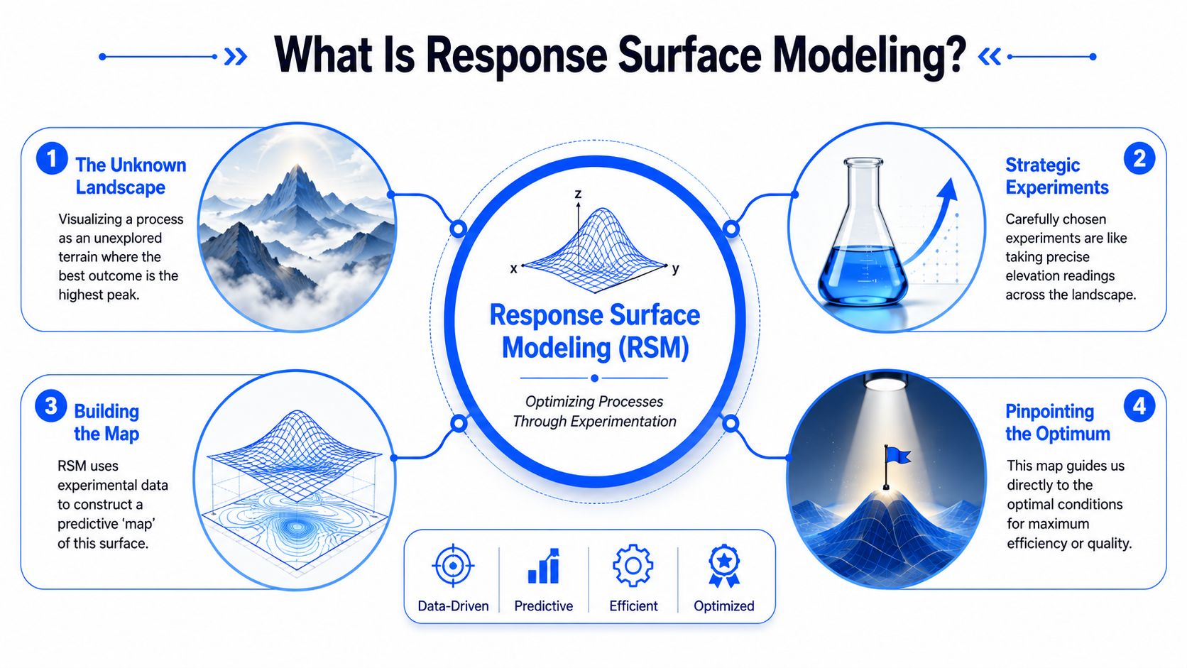
A map for a surface you can't see directly
That “surface” is the relationship between the inputs you control and the output you care about. In RSM language, the inputs are factors and the output is the response. If you're optimizing a coating process, factors might include temperature, pressure, concentration, or line speed. The response might be adhesion, gloss, defect level, or throughput.
The reason this method became so important is historical and practical. Response surface methodology is generally traced to the 1951 paper by George E. P. Box and K. B. Wilson, which formalized the idea of using a sequence of designed experiments to find an optimum response. It emerged from industrial and chemical-engineering needs in the 1950s and introduced a practical framework for modeling curvature and factor interactions with polynomial equations (history of response surface methodology).
That phrase “curvature and factor interactions” is the heart of it. Real processes often don't move in straight lines. A factor can help, then hurt. Two factors can be harmless alone and powerful together. Response surface modeling is built to capture that structure.
A short walkthrough helps anchor the idea:
- Choose the factors you can control reliably.
- Define the response in a way the lab can measure consistently.
- Run a designed set of experiments across a chosen region.
- Fit a mathematical surface that predicts the response between tested points.
Later in the workflow, that fitted surface becomes a decision tool.
A visual explanation helps if you're training colleagues or aligning a cross-functional team:
The three pieces that matter
Most of the confusion around response surface modeling comes from overcomplicating the math too early. Operationally, only three pieces matter at the start.
| Piece | What it means in practice | Typical examples |
|---|---|---|
| Factors | Inputs you can set on purpose | Temperature, pressure, concentration, speed |
| Response | The output that defines success | Yield, strength, quality, uniformity |
| Surface | A fitted model of how the inputs shape the output | Linear effects, interactions, curvature |
The “surface” part is what makes the method more than a standard DoE summary. You're not only estimating whether a factor matters. You're estimating how the response bends as factors move together.
A useful mental model is this: every run is a point, but the decision is made on the shape between the points.
That's why response surface modeling still fits so well inside modern AI and ML tools. Many advanced platforms are doing a more automated, larger-scale version of the same core task. They learn from sampled points, fit a predictive approximation, and recommend where to probe next. The terminology may shift toward surrogate models or experiment planning engines, but the foundation is recognizable.
Choosing Your Experimental Design for RSM
The design choice is where many projects either become efficient or become wasteful. A good response surface study isn't just about fitting a quadratic model later. It starts with selecting a design that matches how your lab operates.
Start with the job the design needs to do
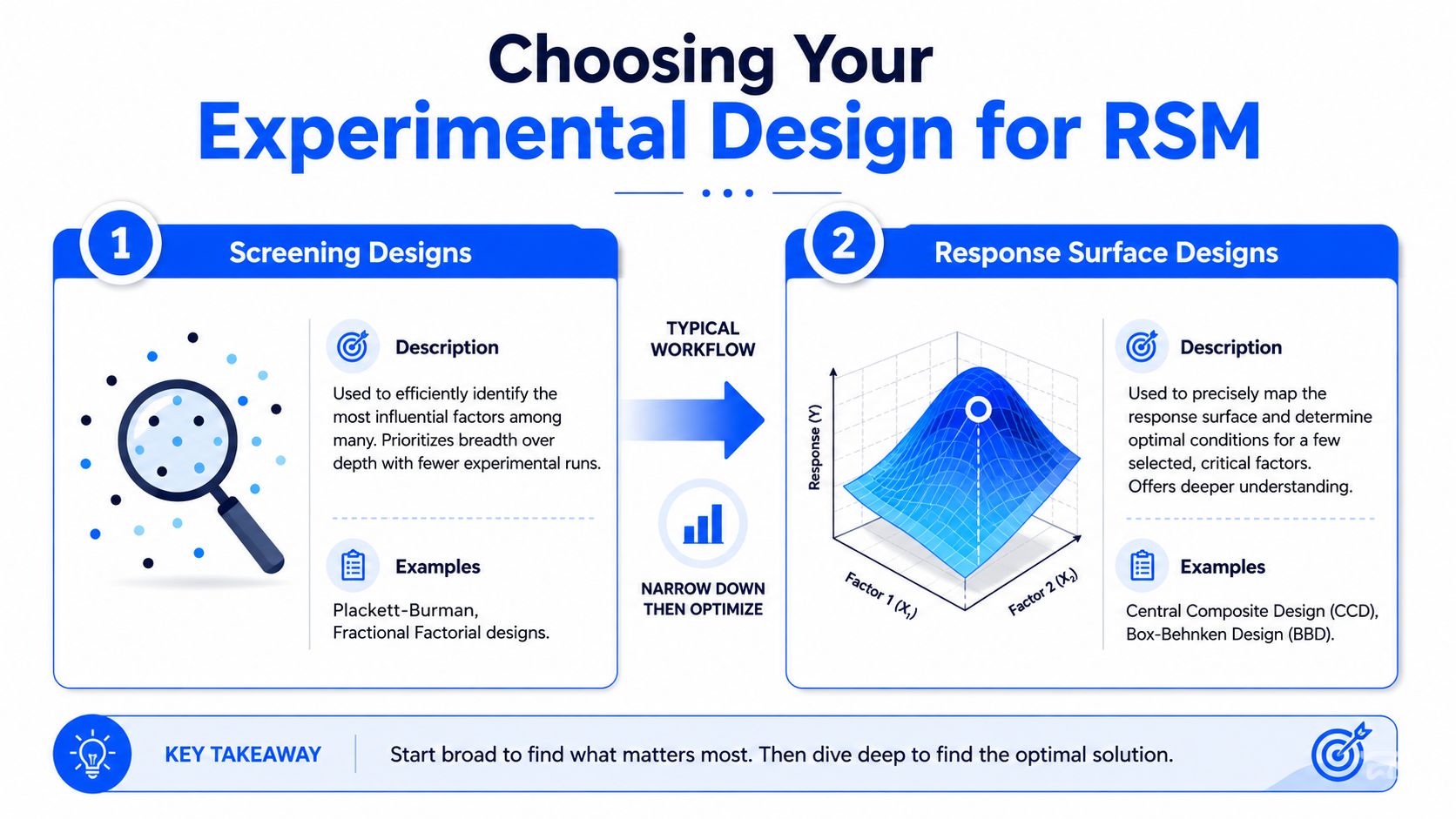
Some teams jump into a response surface design before they've narrowed the factor list. That usually creates noise. If you still have many possible variables, screening designs come first. Once the field is narrowed to the few factors that determine the response, then response surface designs earn their place.
A major reason RSM remains influential is efficiency. It's designed to explore curvature and interactions with fewer runs than exhaustive testing, and the workflow often starts with a first-order model to find the direction of improvement before moving to a second-order design such as Central Composite Design or Box-Behnken Design to locate the optimum (overview of the RSM workflow).
That sequence matters in budget terms. If you don't yet know where the promising region is, don't spend your best design on the wrong neighborhood.
CCD versus Box-Behnken in practice
Once you're ready for a second-order model, the practical choice usually comes down to CCD or Box-Behnken.
| Design | When it fits well | Trade-off to watch |
|---|---|---|
| Central Composite Design | Good for sequential work and for teams that want a classic path from local exploration into quadratic modeling | Can push you toward more extreme factor settings, which may be hard or risky in some labs |
| Box-Behnken Design | Useful when you want to avoid experimental corners or extreme combinations | Less natural if your team is building directly from an earlier factorial-style exploration |
CCD tends to work well when the team wants continuity from earlier experimentation. You can build from a simpler design, add axial points and center runs, and extend the study without starting over. That's attractive in process development, where the first set of experiments often teaches you enough to justify a more targeted second pass.
Box-Behnken often becomes the better choice when corner conditions are undesirable. That can happen in polymer, chemical, and formulation work where the most extreme combinations are unstable, unsafe, or not meaningful to production.
A few practical selection criteria make the choice easier:
- Use CCD when you expect to build sequentially and may want stronger visibility into curvature near the expanded region.
- Use Box-Behnken when your team needs to stay away from edge conditions.
- Pause and rescope if neither design fits the operating window. That's often a sign the factor ranges need work more than the design type does.
Don't choose a design because it's standard in the software menu. Choose it because the resulting runs are feasible, informative, and defensible to the people who have to execute them.
Good RSM planning is less about textbook purity and more about experimental realism. A design that your operators can run consistently will beat a theoretically elegant one that creates unreliable edge conditions.
Fitting the Model and Checking Its Health
The expensive mistake in RSM rarely happens during design selection. It happens after the runs are complete, when a team fits a quadratic model, sees a smooth surface, and treats it like a process map. That is how weak models get promoted into decision tools.
A fitted response surface is usually a second-order model because it gives enough structure to describe the three effects that matter in real development work: directional effects, factor interactions, and curvature. In practical terms, that means one equation can capture whether temperature helps, whether temperature only helps at certain catalyst levels, and whether the gain peaks before the top of the studied range.
Penn State's overview of second-order RSM lays out that structure clearly. A model can include main effects, squared terms, and cross-terms such as Pressure, H2/WF6, Pressure^2, and Pressure×H2/WF6, which is why quadratic models can reveal turning points and interactions that a first-order fit will miss (second-order response surface modeling).
What the fitted equation is telling you
Each term has an operational meaning:
- Main effects show the average direction of a factor's influence across the studied region.
- Interaction terms show that one setting changes the effect of another.
- Quadratic terms show bending in the surface, including plateaus, peaks, and diminishing returns.
That breakdown matters because RSM is not just curve fitting. It is a compact decision model. In formulation, process, and materials work, the value comes from turning a limited set of runs into a surface your team can interrogate before spending more samples, machine time, or plant effort.
This is also where classical RSM still fits cleanly into modern AI workflows. Many AI-driven experiment platforms start with the same question statisticians have asked for decades: can this response be approximated well enough to guide the next experiment? A quadratic surface is often the first interpretable surrogate a team can trust. If it fails basic checks, a more flexible ML model should not get a free pass.
A practical model check before you trust the optimum
Start with model credibility, not software output. A model that predicts neatly and fails diagnostically will waste budget faster than a rougher model that reflects the process accurately.
In lab and pilot reviews, I use a short set of checks:
- Test whether the overall model explains meaningful variation. If the fit is weak, optimization should wait.
- Inspect the active terms in context. An interaction can matter more than a large standalone coefficient if it changes how the process must be run.
- Compare the fitted shape with the raw observations. If the surface looks smoother than the experiment felt, investigate why.
- Review residual plots. Patterned residuals often point to missing curvature, drift, variance changes, or an omitted factor.
- Check where the predicted optimum sits. A peak near the edge of the design space is a prompt for follow-up runs, not a production recommendation.
Common failure mode: the software reports an optimum at the boundary, but the team only has sparse data there and knows the process becomes unstable near that corner.
ANOVA and regression diagnostics help because they separate signal from convenience. The goal is to confirm that the fitted terms are doing explanatory work, not just absorbing noise. NIST's Engineering Statistics Handbook covers this well in its treatment of response surface designs and model fitting, including the need to examine residuals and lack-of-fit before acting on the model (NIST handbook on response surface methodology).
There is a real trade-off here. Simpler models are easier to explain, easier to defend, and often good enough for local optimization. More flexible AI or ML surrogates can capture messier behavior, but they can also hide poor experimental coverage behind better apparent fit. The strongest R&D teams use RSM as a baseline discipline. If the classical model fails, they learn why. If it holds, they gain a fast, interpretable surface that can anchor the next round of algorithm-guided experimentation.
Interpreting Your Model to Find the Optimum
A team usually reaches this stage with pressure building. The model is fit, the plots look clean, and someone asks for a setpoint to hand to the lab or plant. That is the moment to slow down and interpret the surface like an operating map, not a beauty contest for the highest predicted value.
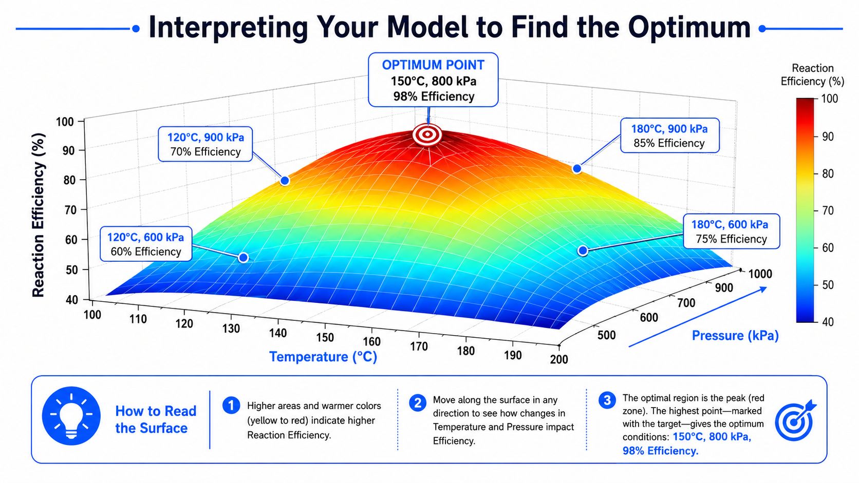
Contour plots and 3D surfaces help because they make the trade-offs visible. A scientist can see curvature, an engineer can judge process sensitivity, and a project lead can decide whether the predicted gain is worth another round of experiments. That shared view is one reason classical RSM still matters inside modern AI-driven R&D platforms. Many newer systems still rely on the same basic logic. Build a useful local approximation, inspect the shape of the response, then choose the next experiment with intent.
How to read the surface
A contour plot works like a topographic map. Closed loops often indicate a local maximum or minimum. Elongated contours usually signal interaction between factors. A saddle means one direction improves the response while another degrades it.
The practical question is not whether the plot looks smooth. The practical question is what kind of decision the shape supports.
- A ridge suggests several near-equivalent settings. That can help when raw material availability, cycle time, or scale-up limits one factor.
- A narrow peak may deliver the highest predicted response, but small execution errors can push the process off target.
- A broad plateau often has more operational value than the mathematical maximum because it gives production a wider margin for normal variation.
A simple reading guide helps keep interpretation disciplined:
| What you see | What it usually means | What to do next |
|---|---|---|
| Circular closed contours | A localized optimum may be present | Check that the point sits comfortably inside the tested region |
| Diagonal contours | Two factors are interacting | Evaluate them together, not one at a time |
| Flattened surface near the top | There may be a stable operating window | Favor settings that balance response with manufacturability |
| Sharp edge optimum | The model is pushing toward a boundary | Plan follow-up runs before changing process specifications |
The highest point on the plot is not automatically the best operating choice. In production settings, teams usually want a condition that holds up to normal shifts in feedstock, operators, instruments, and ambient conditions. A slightly lower response at a more stable setting is often the better business decision.
This is also where RSM connects cleanly to machine learning workflows. AI-based experiment planners often search across many candidate conditions, but they still need a surface worth trusting in the region they recommend. Classical RSM gives teams an interpretable baseline. If a simple quadratic surface already explains the local behavior, use it. If the shape is more irregular, that is a reason to expand the design or bring in a more flexible surrogate, not a reason to skip interpretation.
Why confirmation runs still matter
A predicted optimum is still a prediction. Confirmation runs test whether the process can deliver that result under normal operating conditions.
In practice, I treat confirmation as a decision gate. Run the predicted point, then run one or two nearby settings that a plant or pilot line could maintain without strain. That small step does two jobs at once. It checks the model, and it shows whether the recommended region is usable outside the idealized conditions of the design.
The U.S. National Institute of Standards and Technology emphasizes this same discipline in its treatment of response surface methods, including the use of contour plots, stationary point analysis, and follow-up experimentation before acting on an estimated optimum (NIST Engineering Statistics Handbook on response surface methodology).
Teams that skip confirmation usually pay for it later. They lock onto a point estimate, transfer it too quickly, and then spend time explaining why the gain disappeared in the next batch. Teams that confirm the region learn faster. Sometimes they verify the recommendation. Sometimes they find that the actual opportunity is a nearby setting with slightly lower peak performance and much better day-to-day consistency.
RSM in Action A Polymer Formulation Case Study
The problem the team was actually facing
Consider a polymer formulation team developing a new adhesive. They care about one response above all: peel strength. Two factors appear central from prior screening work, tackifier resin concentration and curing temperature.
Their earlier habit was familiar. Change resin concentration while holding temperature fixed. Then hold resin concentration fixed and try several curing temperatures. The results looked inconsistent because they were inconsistent. The best temperature wasn't constant across the formulation range.
So the team switched to a response surface approach and built a Central Composite Design around the working region they believed was safe and relevant. That gave them a compact experimental plan that could support a quadratic model instead of another round of disconnected trial runs.
What the model changed
Once they fit the model, the key insight wasn't just where peel strength peaked. The key insight was the interaction. At lower resin concentration, increasing curing temperature helped. At higher resin concentration, the same temperature increase eventually became counterproductive. OFAT work had blurred that pattern because it kept resetting one variable while overlooking the changing effect of the other.
The contour plot made the practical choice obvious. There wasn't a single “best temperature” for the adhesive. There was a best temperature region conditional on resin loading.
That changed how the team made decisions:
- They stopped arguing about which single factor “mattered most.”
- They identified a narrower formulation window worth scaling.
- They planned confirmation runs near the modeled sweet spot instead of repeating broad exploratory work.
This kind of case is why response surface modeling fits formulation science so well. Polymer systems rarely reward isolated thinking. Viscosity, cure, compatibility, and final properties all tend to move together. A surface model won't remove that complexity, but it will make the complexity visible.
The broader lesson is practical. A well-run RSM study doesn't just point to an optimum. It tells the team why the optimum sits there, what trade-offs surround it, and how sensitive the recommendation is to changes in the inputs.
The Next Evolution RSM in an AI-Driven World
Why classical RSM still matters inside modern platforms
Some teams talk about AI as if it replaces classical experimental design. In practice, the opposite is closer to the truth. Modern AI-driven R&D systems often depend on the same logic that made response surface modeling valuable in the first place: sample intelligently, build a predictive approximation, and use that model to choose the next experiment.

For teams working across formulation, process, and scale-up, the key upgrade is workflow integration. Instead of running a one-off DOE in a statistics package and leaving the results in a slide deck, modern systems can connect design selection, historical experiment data, model fitting, and next-step recommendations in one environment.
Where AI changes the workflow
Platforms like Polymerize become relevant as operational infrastructure rather than as a replacement for statistics. The platform includes DOE capabilities for materials R&D, and in an AI-native workflow that matters because the design and analysis can sit alongside broader experimental history, predictive models, and formulation knowledge rather than staying trapped in a single study.
AI also helps where practitioners usually lose time. It can organize fragmented datasets, suggest which variables are worth modeling together, and compare the local RSM result against wider project history. For teams that want broader support around analysis, these AI statistical analysis tools are also useful to review because they show how fast the tooling layer around experimental interpretation is evolving.
The important point is simple. Classical response surface modeling is still foundational. AI makes it more continuous, more connected, and more scalable across an R&D organization.
If your team is trying to get more out of limited experimental budgets, Polymerize is one option for bringing DOE, experimental data, and AI-guided formulation work into a single workflow so scientists can plan the next experiment with more structure and less guesswork.

