You've finished a formulation study. The spreadsheet is clean, the regression is run, and the output looks important. Then you hit the same wall most lab teams hit: a coefficients table full of signs, decimals, p-values, and fit statistics that don't tell you, at a glance, what to do on Monday morning.
For materials R&D, that last step matters most. You don't need regression to impress readers in a report. You need it to answer practical questions. Should you raise the coupling agent? Is cure temperature driving hardness, or just moving with another process setting? Is this model strong enough to guide the next design of experiments, or is it only describing noise in a narrow data set?
That's the core job of regression interpretation in a lab setting. Translate statistical output into decisions about ingredients, processing conditions, and the next experiment. When people learn how to interpret regression results in that context, the output stops being a passive summary and becomes a screening tool for where to spend scarce bench time.
Table of Contents
- Start with the coefficient
- Use p-values to judge evidence strength
- Let confidence intervals set the risk level
- Residuals are model quality control
- Multicollinearity confuses interpretation
- Data integrity matters before statistics do
From Raw Data to Real Insights
Most regression mistakes in R&D don't come from the software. They come from reading the output in the wrong order.
A chemist runs a model on tensile strength, includes resin ratio, filler loading, mixing time, and cure temperature, then jumps straight to whatever variable has the smallest p-value. That's understandable, but it's not enough. A useful interpretation starts with the question the experiment was meant to answer, then checks whether the model result is both statistically credible and experimentally actionable.
In materials work, the action is rarely abstract. You're deciding whether to shift a formulation window, tighten a process control band, drop a factor from the next DOE, or collect better data because the current model isn't trustworthy.
Use the output in the order decisions happen
A practical reading order looks like this:
- Look at the coefficient signs first. They tell you whether increasing a factor is associated with higher or lower response.
- Check p-values next. That tells you whether the observed association is supported strongly enough to treat as evidence rather than a fluctuation.
- Review the confidence interval. That tells you how precise the estimated effect is.
- Assess model fit. A significant variable inside a weak model can still mislead your next experiment.
- Run diagnostics. If assumptions fail, the table can look clean while the conclusions are wrong.
Practical rule: Don't ask “Is this factor significant?” first. Ask “If this result is real, what would I change in the lab?”
That one shift improves interpretation immediately. It forces you to connect the math to controllable variables. A positive coefficient for a toughening agent may suggest you should test a higher level. A wide interval around that effect may suggest you shouldn't spend a full round of confirmation work yet. A low-explanatory model may suggest the underlying driver isn't in the dataset at all.
Regression isn't the finish line. It's a filter between a completed experiment and a better one.
Decoding Coefficients P-Values and Confidence Intervals
The coefficients table translates statistical output into formulation and process decisions.
In a materials lab, that usually means questions like these: if we raise filler loading, does hardness move enough to matter? If mixing speed shows a negative effect on viscosity, is that a real process lever or noise from a small dataset? The table helps answer those questions when you read each column for its job, then combine them before changing the next experiment.

Start with the coefficient
The coefficient is the estimated change in the response for a one-unit increase in a predictor, while the other modeled predictors are held constant. Jim Frost's discussion of interpreting coefficients and p-values in regression is a good reference for the mechanics. In practice, chemists and materials scientists should focus on whether the sign and size point to an actionable lever.
Suppose your response is hardness and one predictor is filler loading. A positive coefficient means higher filler loading is associated with higher hardness within the tested design space. That supports testing the high end of the studied range or planning an expansion step if the gain looks useful.
Use caution here. A positive coefficient does not overrule processing limits, brittleness risk, dispersion problems, or cost. Regression estimates the trend inside the region you tested. It does not certify what happens outside it.
A practical read looks like this:
- Positive and large enough to matter: Consider increasing the factor in the next DOE or confirmation run.
- Negative and large enough to matter: Consider reducing the factor, or check whether it protects another property you still need.
- Near zero: Treat it as a low-priority lever unless mechanism or prior work says otherwise.
Use p-values to judge evidence strength
The p-value helps you judge whether the estimated effect is supported strongly enough to treat as evidence rather than random variation. Many teams use a conventional cutoff such as 0.05. That can be a useful screening rule, but it is still a screening rule.
For R&D decisions, the main mistake is treating statistical significance as the same thing as formulation importance. A tiny effect can produce a low p-value in clean data and still be irrelevant to production. A large estimated effect can miss the cutoff because the experiment had too few runs, too much measurement noise, or too narrow a factor range.
That distinction matters in the lab:
- Low p-value, small coefficient: The factor is probably real, but it may not justify reformulation work.
- Higher p-value, sizeable coefficient: The factor may deserve another targeted experiment with tighter measurements or a wider range.
- Borderline p-value with a plausible mechanism: Keep it in play if the chemistry supports it.
Use p-values to grade evidence, not to make the entire decision for you.
Let confidence intervals set the risk level
The confidence interval shows the range of effect sizes still plausible given your data. For experimental planning, this is often the most useful part of the table because it tells you how wrong the point estimate could be. If you want a plain-language refresher on interval thinking, this guide to confidence intervals for marketers is surprisingly useful because it focuses on interpretation rather than formula memorization.
A tight interval that stays positive gives you a clearer basis for action. A wide interval means the coefficient may be pointing in the right direction, but the uncertainty is still large enough to make the next formulation choice risky.
For materials work, confidence intervals help answer questions like these:
| Output pattern | What it usually means in R&D | Likely next move |
|---|---|---|
| Positive coefficient, low p-value, tight interval | Strong candidate driver | Confirm and optimize |
| Positive coefficient, higher p-value, wide interval | Signal may be real but uncertain | Add runs or improve measurement |
| Negative coefficient, low p-value | Likely penalty factor | Reduce level or constrain process window |
| Interval near zero | Effect may be too small or too uncertain | Prioritize other variables |
Read the three pieces together. The coefficient tells you direction and estimated size. The p-value tells you how strong the evidence is. The confidence interval tells you how much decision risk remains. That combination is what turns a regression table into a useful next experiment.
Assessing Overall Model Fit with R-Squared
A model can contain a few interesting coefficients and still be poor at explaining the system.
That's why you need R-squared, or R², which is the standard measure of how much variation in the outcome a regression model explains, and it ranges from 0 to 1. JMP's overview of interpreting regression results gives a concrete example: an R² of 0.489 means the predictors explain 48.9% of the variance in the dependent variable.
What R-squared tells you in a lab setting
For materials scientists, R² answers a practical question: how much of the property variation your model is capturing.
If your response is viscosity and your model includes solvent ratio, solids content, and mixing speed, R² tells you how much of the observed viscosity spread those variables explain together. It doesn't tell you whether the model is causal. It doesn't prove you included the right physics. It tells you how much of the variation is accounted for.
That matters because a coefficient inside a weak explanatory model deserves more caution than the same coefficient inside a model that captures the system well.
What counts as good depends on the problem
There is no universal “good” R² for R&D.
In exploratory formulation work, lower explanatory power can still be useful because the chemistry is messy, measurement conditions vary, and critical variables may still be missing. In a stable manufacturing process with tighter controls, you'd usually expect a stronger fit before using the model to guide process limits.
A very high R² can also be a warning sign. In small experimental datasets, especially when many predictors are stuffed into one model, the fit may look excellent because the model is memorizing quirks of the current runs rather than learning a stable relationship.
That's where adjusted R-squared becomes helpful. When you compare models with different numbers of predictors, adjusted R-squared is more reliable because it penalizes unnecessary complexity. If adding a variable barely changes practical interpretation and doesn't improve adjusted fit, it may be clutter, not insight.
The most useful model in formulation work is rarely the one with the longest variable list. It's the one that explains enough variation to guide the next experiment without pretending to know more than the data support.
Use R² to judge how much confidence to place in the model as a whole. Use adjusted R² when you're deciding whether another variable belongs in the model at all.
Essential Diagnostic Checks for Reliable Results
A regression table can look polished while the model underneath is unstable.
That's why diagnostics are the quality control step. Before you act on a coefficient, make sure the model assumptions aren't being violated in ways that distort the result.
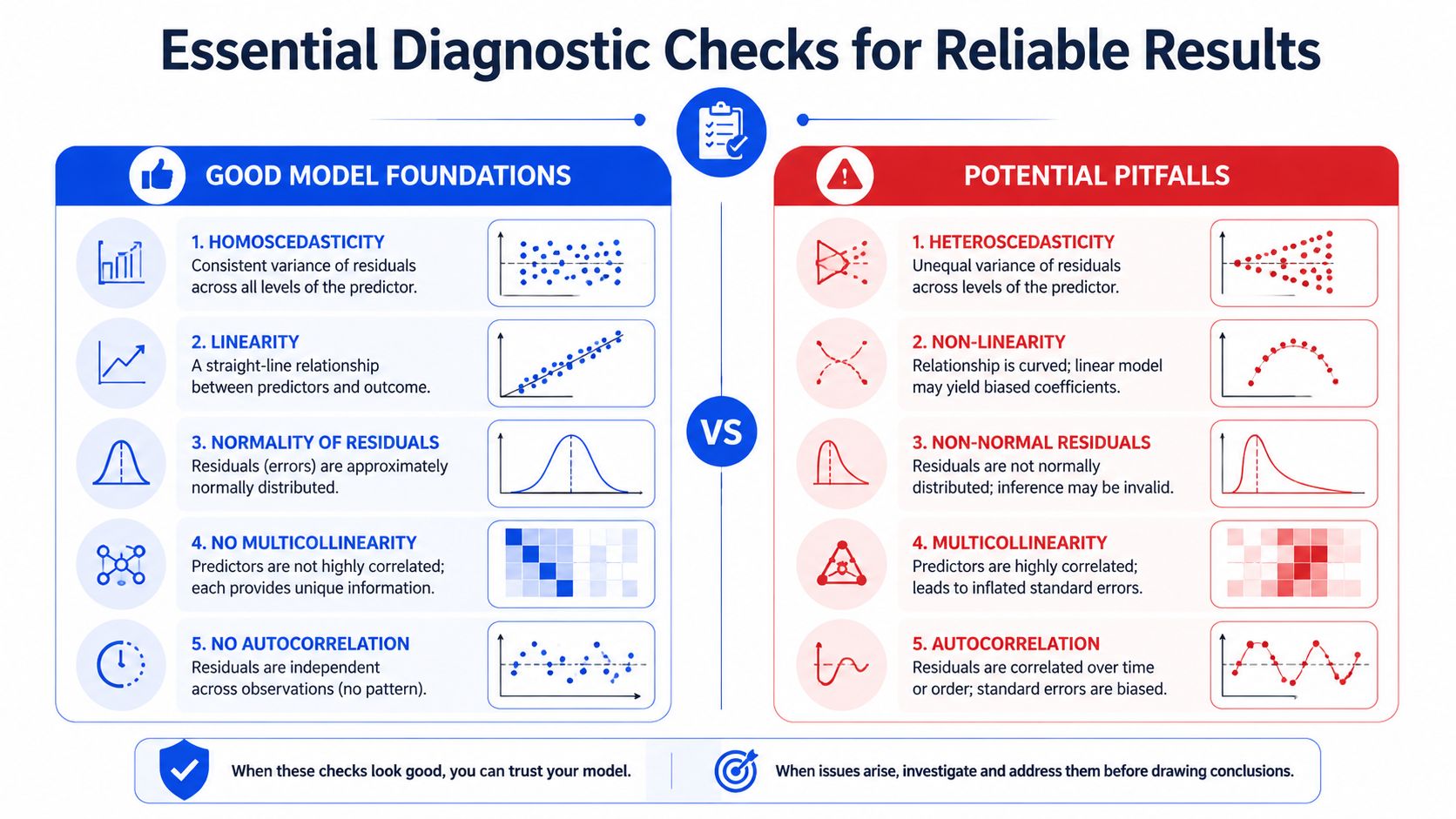
Residuals are model quality control
Residuals are the differences between observed values and model-predicted values. They tell you what the model is missing.
When residuals scatter randomly around zero, that's a good sign. When they form a pattern, the model is often wrong in a specific way. Minitab's approach, referenced in the JMP material discussed earlier, recommends checking residual plots to confirm assumptions. That advice is especially important in formulation and process development, where curved relationships and variance changes are common.
Look for these patterns:
- Curved pattern: The relationship may not be linear. Your model may need transformed variables, interaction terms, or a different functional form.
- Funnel or megaphone shape: Variance changes across the prediction range. In lab terms, your model may be more reliable for low-viscosity or low-strength samples than for high ones.
- Clusters: You may have hidden batches, operators, raw material lots, or instrument states in the data.
- Extreme outliers: Check whether they're chemistry, process upset, transcription error, or measurement failure.
A short visual explanation often helps teams align on what to inspect:
Multicollinearity confuses interpretation
Some predictors move together so closely that the model struggles to separate their individual contributions.
In materials work, this happens all the time. Two plasticizers may rise together across legacy experiments. Solids content and viscosity may be tightly linked because operators adjusted one in response to the other. Temperature and line speed may have changed together during process troubleshooting.
When that happens, coefficient estimates can become unstable. One variable may appear important in one model specification and less important in another, not because the chemistry changed, but because the data don't contain enough independent movement to separate the effects cleanly.
A simple way to think about multicollinearity:
| Situation | What the model experiences | What you should do |
|---|---|---|
| Two ingredients serve similar roles | Redundant information | Reduce overlap in next DOE |
| Process settings always changed together | No clean separation of effects | Decouple factors experimentally |
| Derived variables duplicate raw variables | Inflated uncertainty | Keep the more interpretable representation |
Lab advice: If two inputs always travel together, the model can't tell you which one deserves the credit.
Data integrity matters before statistics do
Many regression problems are not statistical problems first. They're data problems.
If batch IDs are inconsistent, units shift between runs, manually copied values get rounded, or test methods changed mid-study, diagnostics will surface the symptoms but not fix the cause. The habit is the same whether you work in regulated labs or modern digital analytics: trace the origin of the number before trusting the model built on top of it. That's why the ALCOA principles still resonate outside pharma, and this piece on ALCOA data integrity for marketing is useful because it translates core integrity habits into another data-heavy operating environment.
For day-to-day model checking, use this short checklist:
- Check residual plots early: Don't wait until after you've written conclusions.
- Review factor coupling: Ask whether predictors were independently varied or merely co-recorded.
- Inspect outliers with context: Pull notebooks, instrument logs, and lot records.
- Confirm measurement consistency: A clean model can't rescue mixed test methods.
Good diagnostics don't just protect the analysis. They prevent the next experiment from being built on a false story.
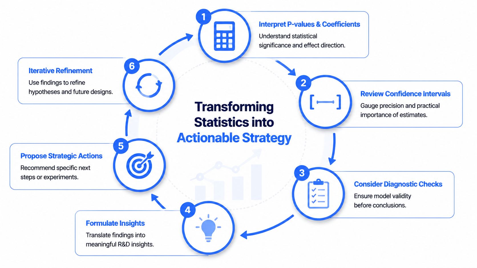
From Statistics to Strategy for Your Next Experiment
The value of regression in R&D shows up only when it changes experimental choices.
A model output should lead to a concrete next step: expand a factor range, remove a weak variable, redesign the DOE, tighten a process variable, or collect better data before making any formulation decision.
A practical decision framework
In lab meetings, the most useful discussion usually starts with “Given this output, what do we do next?” These rules work well.
- If a factor shows a clear positive effect and the estimate is precise, treat it as an optimization lever. Move deliberately toward the better region and confirm the gain in a follow-up study.
- If a factor looks promising but uncertain, don't over-interpret. Add targeted runs around that variable, improve measurement repeatability, or widen the explored range.
- If a factor carries a clear negative effect, constrain it. That may mean lowering its level, narrowing its processing window, or using it only when another property target justifies the trade-off.
- If a factor remains uninformative, stop giving it center stage. Remove it from the next DOE unless process knowledge says it must remain.
Many teams waste time. They keep weak factors in every new design because “we've always tracked them.” Regression should help you retire passengers and focus on drivers.
How to convert output into DOE choices
Treat the model as a map of where uncertainty still lives.
If the model suggests one ingredient matters more than another, the next DOE shouldn't spread effort evenly. Give more design resolution to the factors that appear to drive the response, especially where chemistry and the data tell the same story.
A practical conversion might look like this:
- Rank factors by actionability, not just statistics. A controllable ingredient with a stable signal is more useful than a noisy environmental variable you can't manage.
- Separate optimization from discovery. If the model fit is decent and diagnostics are clean, optimize. If fit is weak or residuals show structure, return to discovery mode.
- Probe suspected interactions experimentally. If two variables seem entangled, build the next design so they vary independently.
- Use replicate runs strategically. When uncertainty is high, replication often teaches more than adding another loosely chosen factor.
Strong regression interpretation ends with a changed experiment plan, not a highlighted spreadsheet.
Another good habit is to decide what would falsify the current conclusion. If you believe filler loading is the key driver, what result in the next set of runs would prove that belief wrong? That mindset keeps teams from turning one model into doctrine.
When people ask how to interpret regression results for materials R&D, the answer is different from generic statistics advice. The point isn't just to identify significance. The point is to decide whether to increase an ingredient, constrain a process variable, simplify the design space, or admit that the current experiment didn't capture the actual mechanism.
Communicating Your Findings to Stakeholders
A strong analysis can still fail if you present it as a dense output table.
Project managers want to know what changes. Business leaders want to know what risk remains. Other scientists want to know whether the conclusion is solid enough to build on. None of those audiences benefit from a screen full of coefficients without interpretation.

Lead with the decision not the table
When you report regression output, start with the recommended action.
Say, “Increase additive A in the next formulation window and hold process temperature tighter because both appear to be the most credible drivers.” Then support that recommendation with the statistical evidence and the diagnostic caveats. That sequence is far easier for non-specialists to follow than starting with p-values and hoping they infer the recommendation themselves.
Good communication also separates three ideas that often get mixed together:
- What the model suggests
- How confident you are
- What you want the team to do next
If any one of those is missing, stakeholders either overreact or tune out.
A one-slide summary that works
A single summary slide or page should include:
| Slide section | What to include |
|---|---|
| Question | The response property and the business or technical decision tied to it |
| Main drivers | The few factors that look most influential, with direction of effect |
| Confidence | Whether the evidence is strong, mixed, or uncertain |
| Model reliability | A short note on fit and diagnostics in plain language |
| Recommended next step | Specific experiment, confirmation run, or process change |
| Risk note | What could still change the conclusion |
Keep the language concrete. “Cure temperature appears directionally important, but the estimate is still uncertain, so we recommend a focused follow-up DOE” is stronger than “temperature was marginally significant.”
Your stakeholders don't need every model detail. They need a reliable recommendation, the reason behind it, and the boundary conditions around that recommendation.
That's the final skill in learning how to interpret regression results. Not just reading the output, but turning it into a decision narrative other people can trust.
If your team is trying to turn scattered experimental results into faster, more reliable materials decisions, Polymerize is worth a look. It helps R&D organizations unify fragmented lab data, apply explainable models to formulations and process variables, and plan the next experiment with more confidence instead of relying on trial and error.

