



Your formulation model is ready to predict glass transition temperature, but the dataset isn't. In a 24-run epoxy design of experiments, 11 runs have no DSC trace. The instrument was being calibrated, three samples cracked during preparation, and one technician forgot to save a file. The team now has to decide whether to discard rows, enter zeros, or rerun experiments that consume time and material.
That decision isn't routine cleanup. Missing value imputation changes which evidence enters the model, how uncertainty is represented, and sometimes the scientific conclusion itself. For materials teams, the right question isn't, “Which algorithm fills the blanks?” It's, “Why is each value missing, what information remains available, and what decision will depend on the completed dataset?”
Table of Contents
- MCAR means the gap is unrelated to the data
- MAR uses information you can observe
- MNAR depends on the unobserved value
- Simple fills establish a baseline
- Statistical methods represent relationships and uncertainty
- Flexible models can capture chemistry, but they can also memorize it
- Hide known values before filling unknown ones
- Check whether the completed distribution remains physical
- Test the decision, not just the column
- Myth one, more rows always solve missingness
- Myth two, imputation removes bias
- Myth three, a clever model excuses leakage
Why Missing Values Stall Materials R&D Projects
A missing DSC result doesn't mean the material has a glass transition temperature of zero. It means the measurement process didn't produce an observed value. Treating those two conditions as equivalent creates a physical and statistical error before modeling even begins.
Start by separating the material, the experiment, and the measurement record. A cracked specimen may indicate brittleness, poor preparation, an unsuitable fixture, or an ordinary handling incident. An absent file may reflect an operator mistake rather than a property of the formulation. The reason matters because the missingness may be related to composition, cure state, viscosity, or laboratory workflow.
Practical rule: Never assign a numerical meaning to a blank until you know what happened at the instrument, sample, and file-record levels.
Why row deletion can distort the campaign
Deleting incomplete rows looks clean, but it can remove exactly the formulations that are difficult to process or characterize. If highly filled epoxies are more likely to crack during preparation, a complete-case dataset overrepresents easy-to-test formulations. The resulting model may describe the laboratory's measurement convenience rather than the chemistry's behavior.
The same issue appears across enterprise R&D. Instrument exports, LIMS records, spreadsheets, ELNs, and handwritten notes often preserve different pieces of the experiment. A missing value can therefore mark a process pathway, not just an empty cell. Campaigns run in one lab may have complete thermal analysis, while another lab records mechanical properties but omits processing details.
Imputation is a scientific assumption
Missing value imputation supplies a plausible value under explicit or implicit assumptions. A mean fill assumes that a typical observation is an acceptable substitute. A regression estimate assumes that observed variables explain the missing measurement. Multiple imputation acknowledges that more than one completed dataset may be plausible.
This history predates modern data platforms. The statistical literature records early examples from experimental field work in the 1930s, formal publication in 1953, and manual card-based imputation in the Canadian Census before modern software existed, as summarized by Schafer and Graham's historical survey. The lesson for materials scientists is straightforward: imputation has always been a method for making assumptions visible, even when those assumptions were implemented by hand.
Before choosing a method, document:
- What is missing: A DSC trace, a scalar extracted from that trace, a process condition, or an entire experiment.
- Why it is missing: Instrument calibration, sample failure, operator error, file-transfer loss, or a result outside the instrument's usable range.
- What is observed nearby: Composition, batch, cure cycle, operator, instrument, and other measured properties.
- What decision follows: Ranking formulations, estimating a property, testing a hypothesis, or reporting an effect.
A completed table is useful only when its provenance and assumptions remain attached.
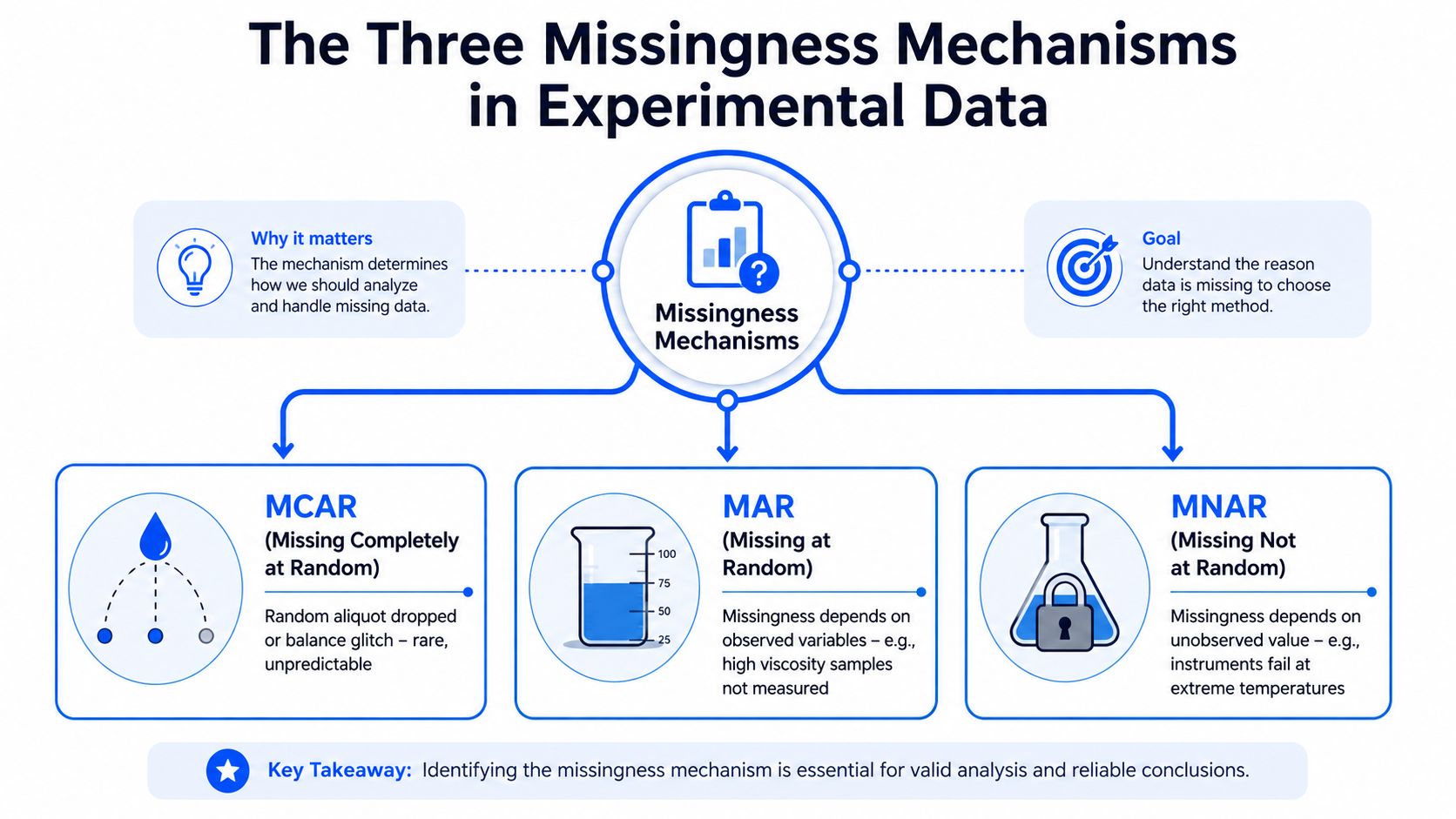
The Three Missingness Mechanisms in Experimental Data
A tensile result disappears after a brittle specimen breaks during mounting. On the same day, a file transfer loses several measurements from one instrument, while high-viscosity samples are more likely to fail preparation. These blanks look similar in a table, yet they imply different assumptions for imputation.
Missingness mechanisms describe how an absent value relates to the process that generated the data. The blank alone cannot identify the mechanism. Analysts infer it from experimental records, instrument behavior, sample history, and relationships among observed variables.
MCAR means the gap is unrelated to the data
Missing completely at random, or MCAR, describes a gap unrelated to the sample, its unobserved result, or other data-generating features. A random aliquot is dropped, a balance briefly glitches, or a file is lost for an unrelated technical reason. Under MCAR, complete-case analysis may be less biased than under other mechanisms, although it still discards usable information.
True MCAR is uncommon in instrument-heavy materials programs. A calibration outage can affect samples run during one shift. A dropped aliquot may be more likely in a high-viscosity formulation. File loss can also become structured when one operator or instrument handled a particular formulation family.
MAR uses information you can observe
Missing at random, or MAR, means missingness depends on variables already recorded. A tensile reading may be absent because the sample was too brittle to mount, while crosslink density, cure temperature, filler loading, or preparation route remains available. Those predictors can support an estimate of the missing result.
MAR still requires careful setup. Instrument identity, operator, batch, and formulation family may explain where gaps occur. Leaving them out can make structured experimental loss appear random, causing an imputation model to misrepresent the formulation space.
MNAR depends on the unobserved value
Missing not at random, or MNAR, occurs when missingness depends on the value that was not observed or on a closely related unobserved condition. A cycle-life result may be absent because a cell shorted before testing. A band-gap measurement may be omitted because the sample did not crystallize. A failure test may go unreported precisely because the specimen failed.
An observed table cannot recover that information by itself. Use a domain model, sensitivity analysis, failure indicators, censored-data methods, repeat testing, or a documented assumption about the unobserved outcomes.
The percentage of missing cells is not enough to choose a method. The mechanism determines what a filled value is allowed to mean.
Create a missingness map before modeling. Compare gaps with formulation family, instrument, operator, batch, sample preparation outcome, and process conditions. Clustering around extreme materials or failed experiments is scientific evidence, not administrative noise. Record that pattern in the enterprise AI workflow so imputation remains tied to provenance, assumptions, and later model decisions.
Comparing Simple, Statistical, and Model-Based Imputation Methods
The best imputation method depends on the geometry of the data and the purpose of the model. A fast median fill may be adequate for a descriptive dashboard. It may be inappropriate when the completed values feed a formulation ranking or a claim about a process effect.
| Method Family | Accuracy on Correlated Features | Uncertainty Handling | Runtime / Cost | Best Use Case in Materials R&D |
|---|---|---|---|---|
| Mean, median, or mode | Low when correlations and groups matter | Poor unless uncertainty is added separately | Very low | A simple baseline, stable low-impact fields, or exploratory analysis |
| Zero or fixed domain value | Appropriate only when zero has physical meaning | Usually poor | Very low | True structural zeros, never generic blanks |
| Regression imputation | Moderate to strong when relationships are stable and specified | Limited for a single fill | Low to moderate | Process variables explained by recorded formulation and cure conditions |
| Multiple imputation | Can represent joint relationships when the model is well specified | Stronger, because results are combined across plausible datasets | Moderate to high | Inference, effect estimation, and decision workflows that need honest uncertainty |
| k-nearest neighbors | Useful for local similarity and correlated features | Weak for a single completed value | Moderate | Small or medium formulation spaces with meaningful similarity metrics |
| Iterative, random forest, or related model-based methods | Can capture nonlinear relationships, subject to overfitting | Depends on the implementation and whether ensembles are retained | Moderate to high | Nonlinear composition-property patterns with enough comparable observations |
| Gaussian process or generative models | Potentially useful for smooth structure or complex latent patterns | Can provide model-based uncertainty, but assumptions require scrutiny | High | Structured surrogate problems where uncertainty and geometry justify the complexity |
Simple fills establish a baseline
Mean and median imputation are easy to inspect, reproduce, and explain. They can be reasonable for a low-impact variable with limited missingness and no meaningful subgroup structure. Median filling is often less sensitive to extreme observations than mean filling, but neither method preserves the original relationships among features.
Zero deserves special caution. It's valid only when zero represents a real state, such as an explicitly recorded absence of an additive. A blank cure-time field isn't a zero-minute cure, and a missing modulus isn't zero stiffness.
Add a missingness indicator when a missing record may carry process information. The indicator doesn't correct bias by itself, but it lets the downstream model distinguish measured values from substituted ones.
Statistical methods represent relationships and uncertainty
Regression imputation uses observed formulation and process variables to estimate a gap. It works best when the relationship is stable, relevant predictors are available, and residual uncertainty is retained rather than hidden behind a single point estimate.
Multiple imputation is more appropriate when the completed values will support inference. It creates several plausible datasets, analyzes each, and combines the results so uncertainty from the missing values contributes to the final estimate. Guidance from the National Center for Education Statistics warns that single imputation treats filled values as observed data and can understate variance. The same guidance reports variance underestimation of about 2% to 10% at 5% nonresponse and 10% to 50% at 30% nonresponse, depending on the setting and method.
Flexible models can capture chemistry, but they can also memorize it
k-nearest neighbors can work well when similar formulations have similar measured properties. The distance function must respect units, scaling, formulation composition, and categorical process variables. An iterative imputer can use relationships among several columns, while random forest methods can capture nonlinear structure.
These methods aren't automatically superior. Small experimental datasets offer limited evidence for complex models, and a flexible imputer can reproduce noise or leak information from validation data. A benchmark spanning 84 classification and regression problems found that no method dominated across all tasks, while a time-series health-data review also found no universal winner. The same research reported compute times from about 10 minutes for MIDAS or KNN to roughly 290 minutes for MICE in one large blockwise-missingness setting, as described in the Frontiers benchmark study.
For materials datasets ranging from tens to several thousand rows, start with interpretable baselines, then earn complexity through validation. Gaussian processes can be valuable when the property surface is smooth and uncertainty matters. Variational autoencoders and other deep generative approaches need enough structured data to justify their assumptions, and they should never be selected merely because they sound advanced.
How to Evaluate Whether Imputation Actually Worked
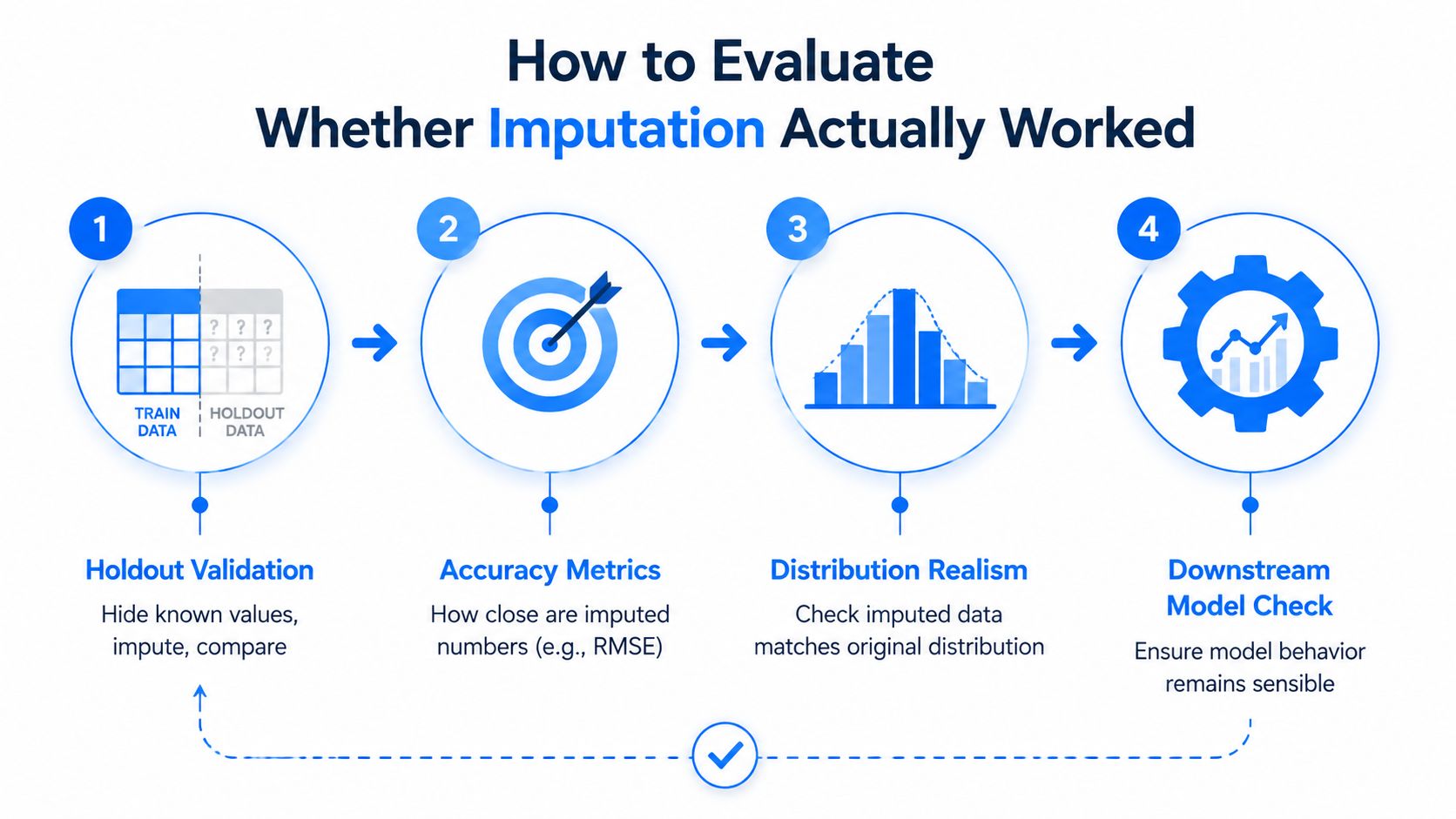
A completed column can look plausible and still damage the scientific task. Evaluate imputation at three levels: numerical accuracy, distributional realism, and downstream behavior.
Hide known values before filling unknown ones
Create artificial missingness by masking observed entries, then run the complete imputation pipeline without allowing the masked values to influence fitting. For continuous properties such as tensile modulus or band gap, compare recovered and original values with RMSE and MAE. For categorical fields such as synthesis route, use classification metrics such as accuracy or F1.
Repeat the masking across relevant subgroups. A method that performs well for low-filler formulations may fail for highly filled systems, a different polymer family, or a specific instrument. Random masking alone can be misleading when real missingness is clustered by batch, operator, time, or failure mode.
Check whether the completed distribution remains physical
Plot observed and imputed values together. Look for a spike at the mean, artificial zeros, compressed tails, implausible ranges, and broken relationships with temperature, composition, or conversion. A low error score can hide a serious problem if the imputer removes the variation that the surrogate model needs to identify candidate formulations.
Consider a kNN estimate for glass transition temperature. It may not be the numerically closest value for every masked row, yet it can preserve local variance and composition-property structure better than a global mean. For an uncertainty-aware surrogate, that structural plausibility may be more valuable than a small improvement in average error.
Test the decision, not just the column
Train the downstream prediction or optimization model using the imputed data and compare its behavior with models trained on appropriate observed subsets. Review ranking stability, calibration, residual patterns, prediction intervals, and sensitivity to the imputation method. If candidate formulations move substantially when you change a reasonable assumption, report that instability.
A short visual explanation can help teams communicate the evaluation logic:
For teams building broader formulation decision systems, a useful adjacent resource is product metadata and scoring with NanoPIM. Product and experiment metadata can reveal whether missingness follows an instrument, batch, or product family, which makes validation more representative.
Pitfalls That Invalidate Imputed Materials Datasets
A formulation dataset may look ready for modeling after every blank has been filled. Yet a missing process condition, failed measurement, or validation leak can make its conclusions unreliable. Imputation works only when the team understands how records became incomplete and keeps that process visible.
Myth one, more rows always solve missingness
A large composition table can still produce a distorted property model when critical processing variables are absent from a systematic subset. Extra rows cannot restore temperature history, cure schedule, crystallinity, or sample-failure information. The model may learn a composition-property relationship that applies only to the best-documented campaigns.
In an enterprise AI platform, attach laboratory, instrument, batch, and campaign metadata before fitting an imputer. This lets the team distinguish broader coverage from repeated records with the same blind spot.
Myth two, imputation removes bias
A mean or regression fill can complete a table without making it representative. If a measurement system records successful runs more reliably than failed runs, a completed dataset can overrepresent successful or easy-to-measure samples, masking the selection process. Inference becomes especially fragile when the filled outcome affects a ranking, release decision, or claim about a formulation variable.
Recent systematic-review evidence illustrates the stakes for substantive conclusions. When missing outcome data were imputed more stringently, the share of meta-analyses whose 95% confidence intervals crossed the null rose from under 4% to 47.9%, and the odds of reversal increased with missingness, reported as OR 1.23 per 1% increase in missing data in the recent review evidence. Materials teams should not transfer those results mechanically to every experiment. The practical warning still applies: imputation can change a scientific conclusion, not only prediction error.
Myth three, a clever model excuses leakage
Fit the imputer inside each training fold. If means, neighbors, regression coefficients, or latent representations are calculated from the full dataset before splitting, validation information enters training. Reported performance then reflects an easier problem than the model will face in production.
| Pitfall / Myth | What Happens | Diagnostic to Run |
|---|---|---|
| More data fixes missingness | Systematic gaps remain systematic, even in a large table | Compare missingness with lab, instrument, batch, formulation family, and process state |
| Imputation eliminates bias | A completed dataset can still overrepresent successful or easy-to-measure samples | Compare observed and missing groups, then run sensitivity analyses |
| Clever models prevent leakage | Flexible imputers still risk absorbing validation information and inflating metrics | Fit every preprocessing step inside the training fold |
| Correlated-column filling is harmless | Imputing one property can create artificial relationships with neighboring properties | Inspect correlation matrices before and after imputation |
| Iterative methods are safe on small datasets | The imputer can overfit experimental noise | Compare against simple baselines and perturb the training sample |
A practical release gate should require provenance, missingness-mechanism assessment, masked-value validation, distribution checks, leakage-safe fitting, and sensitivity to alternative assumptions. Keep those checks in the platform workflow so imputation remains an auditable modeling operation rather than an invisible preprocessing step.
A Polymer R&D Workflow That Recovered an Unusable Dataset
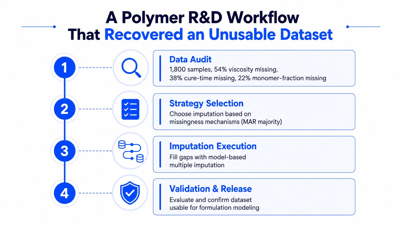
A polymer formulation team inherited a dataset that looked rich but was difficult to model. It contained 1,800 samples, with 54% of viscosity measurements missing, 38% of cure-time readings missing, and 22% of monomer-fraction entries missing. The records came from three laboratories, two LIMS exports, and one handwritten logbook, so a blank could mean a failed measurement, a missing transfer, or a value never recorded.
The audit came before the algorithm
The team first preserved the raw records and added provenance tags for laboratory, source file, operator, instrument, and timestamp. Column-level diagnostics then showed that viscosity gaps clustered around calibration failures, while other missing fields followed particular export formats.
That distinction prevented the team from treating every blank as MAR. Calibration-related gaps required a different response from an unrecorded monomer fraction, and a failed viscosity measurement could carry information about the material or the instrument state.
A tiered strategy matched the data
The team used domain-bounded mean or mode fills for low-impact fields where the substituted value had a clear interpretation. For correlated process variables, they applied per-polymer-family kNN imputation, so neighbors were chemically and operationally relevant rather than merely numerically close.
For the joint behavior of viscosity, cure time, and conversion, they used chained-equation multiple imputation. The approach preserved alternative plausible completed datasets instead of presenting every estimate as if it had been measured.
Each stage ran as a versioned, cached node. The record for every run included the source snapshot, feature set, method, parameters, random seed, and output location. That made it possible to reproduce the dataset and inspect why a particular value had been filled.
Release depended on validation
The team compared observed and recovered distributions, checked ranges and units, and reviewed relationships with polymer family and process conditions. They also evaluated the downstream property-prediction model against a version trained after listwise deletion. The recovered dataset produced a clear improvement in downstream predictive performance, but the team treated that result as evidence of utility, not proof that every imputed value was correct.
The reusable pattern is simple:
- Profile the records and preserve provenance.
- Classify missingness by column and process pathway.
- Impute in tiers, from bounded simple rules to joint model-based methods.
- Validate the values, distributions, uncertainty, and scientific decision.
A large-scale example shows what systematic recovery can look like. In the Fragile Families Challenge dataset, semiautomated processing reduced missingness from 54.63% after initial preparation to 0% at finalization, across 10,423 features and 4,242 rows, using cross-path, cross-caregiver, and cross-year imputation, as reported in the published dataset workflow. That result demonstrates recoverability, not universal safety. Materials teams still need mechanism-aware validation.
Operationalizing Imputation Inside Enterprise AI Platforms
A notebook can demonstrate a method. An enterprise platform must make the method repeatable, inspectable, and governable across instruments, laboratories, and projects.
Start at ingestion
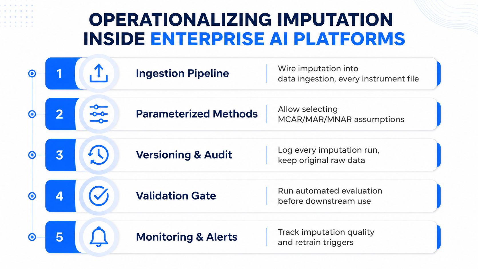
Wire profiling into ingestion for DSC, XRD, tensile CSVs, rheology exports, and LIMS records. The platform should identify schema changes, units, duplicate samples, missingness patterns, and provenance before a downstream model sees the data. Store the imputation model and configuration as lineage alongside the dataset version, not in a scientist's local notebook.
Expose an imputed-versus-measured flag as a first-class field. Chemists should be able to filter candidates by measurement status, compare models trained with and without substituted values, and inspect whether a recommendation depends heavily on imputed inputs.
Preserve uncertainty and explanations
A single completed value hides uncertainty. Multiple-imputation variance, standard errors, ensemble disagreement, or another appropriate uncertainty representation can travel with the estimate into property prediction and candidate ranking.
Explainability should also reach the imputation layer. If a missing cure-time value was estimated from formulation composition, temperature, viscosity, operator, and instrument history, the scientist should be able to inspect those drivers. A SHAP-style view can help, but the interface must distinguish measured evidence from inferred evidence.
Add governance gates
Configure automated checks before imputed data reaches optimization:
- Ingestion profiling: Detect missingness and schema drift for every source.
- Parameterized methods: Record the mechanism assumption, method, feature set, and constraints.
- Versioned audit trails: Retain raw values, imputed values, flags, and run metadata.
- Validation gates: Block or quarantine outputs that fail masked-value, distribution, or physical-plausibility checks.
- Monitoring alerts: Trigger review when missingness patterns, instruments, or formulation families change.
Enterprise R&D also needs an answer when data cannot be pooled. Conventional imputation may be unavailable when files must remain distributed across sites or silos. A 2024 study proposes conditional quantile imputation for distributed data networks and discusses the practical limitation of centralizing files, as described in the PubMed-indexed research. The same direction of work points toward structure-aware methods that use relational or network information when local measurements are weak.
Best Practices for Missing Value Imputation at Scale
Use these rules as a working standard for the next formulation project.
Diagnose the mechanism first. A calibration failure, a brittle specimen, and an unreported failed test aren't interchangeable. MNAR patterns require domain assumptions and sensitivity analysis, not just a more complex estimator.
Use multiple imputation when decisions depend on inference. A single fill is easier to deploy, but it can make estimated values look observed and understate uncertainty. The extra computation is justified when confidence intervals or effect conclusions matter.
Check chemical plausibility before optimizing error metrics. Respect units, ranges, phase behavior, stoichiometry, and instrument limits. A numerically close estimate that violates chemistry is not a successful imputation.
Keep measurement status visible. An imputed-value flag lets models and scientists test whether inferred observations drive a recommendation.
Retrain after process drift. A calibration relationship learned from one instrument state or formulation family may not transfer after a method, supplier, operator, or instrument changes.
Log every run. Save the raw snapshot, feature set, method, constraints, seed, validation results, and output version. Reproducibility is part of scientific evidence.
Treat imputation as a claim. State what you assumed about missingness, what evidence supports that assumption, and how the conclusion changes under plausible alternatives.
Missing value imputation is most useful when it remains connected to experimental reality. The goal isn't to make every table look complete. It's to recover enough structured evidence for a defensible scientific decision while showing where uncertainty and bias still remain.
Polymerize helps materials R&D teams unify fragmented experimental records, operationalize explainable modeling, and keep imputation decisions traceable across formulation workflows. Visit Polymerize to see how your team can turn disconnected lab data into an auditable foundation for better material decisions.
Put your R&D data to work
See how materials teams use Polymerize to plan fewer experiments and reach target properties faster.