



Your coatings team has three years of bake temperatures, solvent blends, catalyst identities, and hardness results stored across spreadsheets. Everyone knows the data contains useful patterns, but nobody can explain which variables drive a pass or fail result, or which experiment should come next. A model that produces only a score won't solve the trust problem.
Decision tree models offer a practical starting point. They turn experimental data into a sequence of questions, such as whether annealing temperature exceeds a threshold or whether solids loading falls below a boundary. That structure resembles the reasoning an experienced formulation chemist already uses, while still exposing where the model's logic is weak.
A tree isn't a magic explanation of chemistry. It is a compact, testable hypothesis about how measured variables divide your historical experiments. Used carefully, it can establish a baseline, reveal useful interactions, and support a closed-loop planning process without hiding every decision behind a black box.
Table of Contents
Why Materials Teams Start with Decision Tree Models
A formulation team usually doesn't begin with a clean machine-learning problem. It begins with an archive of experiments, inconsistent naming, missing process details, and a property that matters commercially. One chemist calls a solvent blend “high aromatic,” another records the individual components, and a third has only a supplier code. The team still needs a useful first model before it can justify a larger data-engineering effort.
A single decision tree is approachable because its prediction can be written as a path. A coating may be classified as passing when the bake temperature exceeds a learned boundary, the catalyst belongs to a particular category, and the solvent ratio remains within a certain range. Each condition can be challenged by a scientist who understands the process.
A natural first model for mixed experiments
Materials datasets combine continuous variables, such as viscosity, temperature, particle size, and molecular weight, with categorical variables, such as polymer family, supplier, catalyst type, and mixing method. Decision trees can work with both types, although categorical encoding still needs to be designed carefully. The model doesn't require the chemist to assume that every relationship is linear or that a one-unit change has the same meaning across the entire formulation space.
That matters in formulation work. A temperature increase may have little effect in one composition region and a large effect in another. A catalyst may matter only when moisture is above a process threshold. Trees represent these conditional relationships through splits rather than through one global equation.
Practical rule: Treat the first tree as a discussion instrument and a benchmark, not as the final authority on mechanism.
The historical record supports that role. Decision-tree development emerged through several advances in recursive partitioning, including AID in 1963, the first classification tree in the THAID project in 1972, and CART, introduced in 1977 and published in book form in 1984. Trees later became building blocks for ensemble methods as the field expanded, as described in this historical review of decision trees.
What the team gains immediately
A tree gives a materials group three useful artifacts:
- A baseline: It establishes whether the recorded variables contain enough signal to predict the target at all.
- A conversation starter: Scientists can inspect the conditions associated with a prediction and compare them with process knowledge.
- A benchmark: Random forests and boosted trees can be evaluated against a simple model rather than in isolation.
CART remains influential because it supports both classification and regression with binary splits. In one crash-severity application, a very large dataset produced similar training and testing accuracy, while comparative work found strong results on some datasets and lower performance on harder ones. The broader lesson is more useful than any individual score. Tree performance depends on feature quality, dataset complexity, and how growth is controlled, as documented in this CART performance study/Z05120207212.pdf).
How a Decision Tree Actually Splits Data
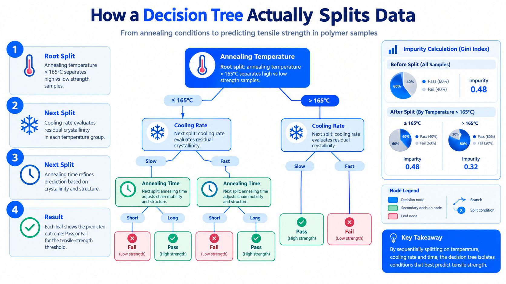
Suppose you're predicting whether a polymer sample passes a tensile-strength threshold. Each row contains annealing temperature, cooling rate, annealing time, catalyst type, and the measured tensile result. The target is binary: pass or fail.
The tree starts with all historical samples in one root node. It searches for a question that divides those samples into two child nodes. A candidate question could be “Is annealing temperature greater than 165°C?” The algorithm tests many possible thresholds and variables, then chooses the split that makes the resulting groups as pure as possible.
Following one sample through the tree
After the temperature split, the high-temperature branch might be divided by cooling rate. A slower cooling rate could separate samples that retain sufficient crystallinity from samples that don't. The algorithm then continues splitting each branch until it reaches a leaf, where it assigns a class such as pass or fail.
For a new formulation, prediction is path tracing:
- Is annealing temperature above the selected threshold?
- If yes, does cooling rate fall on the pass side of its boundary?
- Does catalyst type move the sample into a different terminal group?
- Assign the class stored in the final leaf.
The tree evaluates split quality with measures such as Gini impurity and entropy. Both quantify how mixed the classes are in a node. A node containing almost entirely passing samples has low impurity. A node containing a balanced mixture of passes and fails has higher impurity. The training algorithm chooses the split that produces the greatest reduction in impurity, subject to the growth rules you specify.
Why pruning changes the scientific value
An unrestricted tree can keep splitting until it memorizes unusual experiments, measurement noise, or accidental batch effects. It may produce a perfect-looking explanation for the training spreadsheet and a poor prediction for the next campaign.
You control this risk through pre-pruning, using settings such as maximum depth and minimum samples per leaf. You can also grow a larger tree and apply post-pruning, including cost-complexity tuning, to remove branches that don't justify their added complexity. Depth is also an interpretability control. A depth-3 binary tree can already have up to 8 leaves, and tracing those rules becomes harder as the number of terminal nodes grows, as explained in the tree interpretability discussion.
For a continuous target, the same structure becomes a regression tree. Instead of assigning pass or fail, each leaf predicts a numerical value, often based on the average target value of the training samples that reach it. That makes regression trees useful for properties such as glass-transition temperature, modulus, viscosity, or yield strength, provided the validation design reflects how future experiments will be generated.
Reading Feature Importance Without Fooling Yourself
A feature-importance chart often appears to answer the question every formulation team asks first: which variable matters most? In a standard impurity-based calculation, a feature receives credit for the weighted impurity reduction produced by splits that use it. A variable used near the root affects many samples, while a variable reused in several branches can accumulate credit repeatedly.
That calculation is useful, but it isn't a causal analysis. A composition code with many possible categories can receive inflated importance because it offers many candidate split points. Correlated variables can divide credit unpredictably. A supplier identifier may rank highly because it acts as a proxy for a resin grade, equipment setting, or undocumented process change.
The bias isn't merely philosophical. Research on unbiased split-improvement measures shows that a feature with no predictive power can receive an importance score of zero in expectation after correction, which highlights why raw impurity importance needs scrutiny. The underlying issue is discussed in this ACM study of unbiased feature importance.
| Method | What it measures | Strengths | Weaknesses for materials data |
|---|---|---|---|
| Impurity importance | Reduction in node impurity across tree splits | Fast and easy to inspect | Biased toward high-cardinality variables and unstable with correlated inputs |
| Permutation importance | Performance change after shuffling one feature | Tests reliance on held-out data | Correlated features can mask one another, and results depend on the validation set |
| SHAP values | Contribution of features to individual predictions | Useful for local explanations and interaction review | Explanations can become noisy when the model is unstable or the feature space is redundant |
| Domain review | Chemical and process plausibility of a pattern | Connects model output to mechanism and actionability | Human judgment can favor familiar explanations and miss hidden confounding |
Turning rankings into experiments
Use impurity importance to decide what deserves inspection, not what deserves automatic optimization. If molecular weight ranks below a supplier code, ask whether the supplier variable contains an unrecorded grade difference. If two descriptors describe nearly the same chemistry, don't interpret their ranking order as a meaningful scientific hierarchy.
Permutation importance is most useful when you want to know whether a feature supports held-out predictions. SHAP values help explain why a particular formulation received a prediction, especially when the team needs to inspect both direction and magnitude across samples. Neither method removes the need for grouped validation, careful feature definitions, or a conversation with the scientist who knows how the measurement was produced.
Use the chart to form a question. Use controlled experiments to test the answer.
A feature ranking becomes dangerous when it is copied directly into an experimental plan. The model can identify a predictive relationship, but it can't establish whether changing that variable will change the property, whether the variable is physically controllable, or whether the apparent effect survives a new batch.
Decision Trees Against Random Forests and Boosted Models
A standalone CART tree is often the easiest model to argue with, but it isn't always the most accurate. Random forests average many trees, while gradient-boosted systems such as XGBoost and LightGBM build trees sequentially to correct earlier errors. Linear regression takes a different route, imposing a global relationship that can be valuable when extrapolation matters.
Consider a polymer team with a few hundred formulation records. A single tree may produce a clear rule involving solids loading and cure temperature. A random forest may reduce prediction error substantially, for example by 30% in a hypothetical comparison, but that result is only meaningful if the dataset, metric, and validation design support it. The chemist may still prefer the simpler tree for a Monday planning meeting if the rule can be tested directly.
| Dimension | Single Decision Tree | Random Forest | Gradient Boosted Trees | Linear Model |
|---|---|---|---|---|
| Single-prediction interpretability | High when shallow | Low to moderate through aggregate explanations | Moderate with SHAP, but paths are distributed across trees | High when features and coefficients are stable |
| Nonlinear relationships | Captures thresholds and interactions | Strong | Strong and often more flexible | Limited unless features are transformed |
| Small materials datasets | Useful baseline, but unstable if overgrown | Often more robust than one tree | Can overfit without disciplined tuning | Often competitive when the process is approximately linear |
| Mixed feature types | Works with deliberate encoding | Works with deliberate encoding | Works with deliberate encoding | Requires careful encoding and usually stronger assumptions |
| Training and deployment | Lightweight and easy to serialize | More computational and operational overhead | More tuning and monitoring | Lightweight |
| Extrapolation | Poor outside learned regions | Poor outside learned regions | Poor outside learned regions | Can be useful when the relationship and assumptions support extrapolation |
| Closed-loop explanation | Direct rules can guide experiments | Better for ranking and prediction than direct rules | Strong predictive tool, less direct mechanistic story | Coefficients can support directional reasoning |
Choosing by lab consequence
If the team needs a transparent screening rule, start with a constrained tree. If prediction stability matters more than a single readable path, evaluate a random forest. If the dataset has enough reliable variation and the team can support tuning and monitoring, boosted trees may earn a place in production.
Linear models still deserve a serious test. A formulation group may need to predict outside the historical range, estimate a directional effect, or communicate a compact relationship to process engineering. Trees generally partition the observed feature space rather than describe a smooth law, so they shouldn't be treated as universal replacements for mechanistic or linear models.
The practical workflow is comparative. Fit a simple tree, establish a validation protocol, compare it with a linear model and an ensemble, then decide what kind of error the lab can tolerate. A slightly weaker model that scientists understand and act on can be more useful than a stronger model that nobody trusts.
Three Materials R&D Use Cases That Work Today
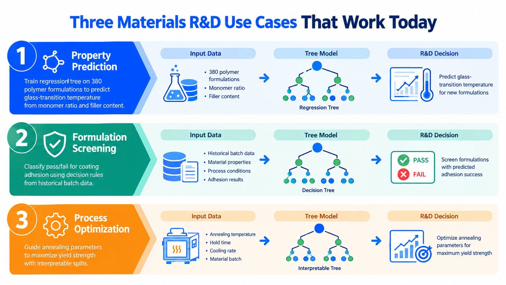
Decision trees become valuable when their output changes a laboratory decision. The following workflows show three different roles, from property estimation to experiment selection.
Property prediction
A polymer group can train a regression tree on 380 historical formulations to estimate glass-transition temperature from monomer composition, molecular weight, and cure schedule, as represented in the workflow concept above. The tree's leaves might correspond to combinations such as a high fraction of one monomer family, a molecular-weight boundary, and a defined cure range.
The researcher doesn't treat the leaf estimate as a new measurement. They use the path to identify which historical formulations are comparable, flag a candidate recipe for synthesis, and decide whether the predicted uncertainty is acceptable for screening. If the prediction depends on a narrow region with few examples, the team may choose a confirmation experiment rather than trusting the estimate.
Formulation screening
For battery cathode slurries, a classification tree can separate pass and fail outcomes using viscosity, solids loading, mixing time, and other recorded process inputs. A leaf rule might identify a region where viscosity is too high when solids loading and mixing conditions combine unfavorably.
The team can invert the rule operationally. Instead of asking the model only whether a proposed slurry passes, the scientist searches for combinations that land in pass-dominant leaves, then checks whether those combinations are chemically feasible, safe, and available for batching. A dashboard that connects the rule to batch records can also support root cause analysis for dashboards when a production or lab outcome deviates from expectation.
Experimental planning
In an active-learning loop, the tree can help identify regions where predictions are uncertain or where the historical design is sparse. The experimental planner proposes a batch of coating experiments, the lab measures the target property, and those results return to the dataset for the next training cycle. The model isn't replacing the chemist's constraints. It is narrowing the set of plausible experiments that deserve attention.
A useful output includes the proposed formulation, the tree path or ensemble explanation, the reason the sample is informative, and the nearest historical precedents. That record lets the researcher distinguish a deliberate exploration from a random trial and makes the next planning meeting more productive.
Preparing Experimental Data the Right Way
Most tree projects fail before model fitting. A split can only be as meaningful as the columns it receives, and materials records often mix chemical identity, process history, batch effects, and measurement artifacts in ways that make accidental shortcuts easy.
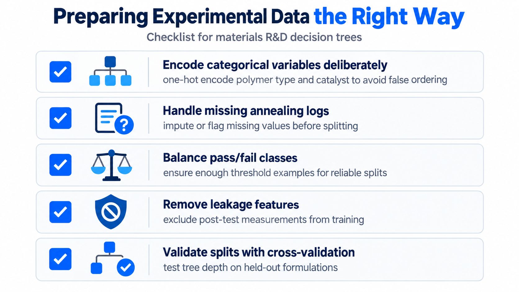
Start with variable definitions. Don't encode polymer type or catalyst identity as arbitrary integers if the numbers imply an order that doesn't exist. Use an encoding strategy appropriate to the implementation, and preserve the original labels in the data dictionary so a future user can understand what each encoded value means.
A practical preparation checklist
- Encode categories deliberately: Treat supplier, catalyst, polymer family, and equipment identity as categorical information rather than pretending that category codes are continuous measurements.
- Inspect skewed variables: Particle size, viscosity, and concentration may have long tails. Review distributions and consider transformations when extreme values would create unstable thresholds.
- Keep replicate information visible: Average replicates only when the scientific question supports averaging, and retain replicate count, spread, and measurement-quality flags. Separate rows can preserve useful variation when each run represents a meaningful observation.
- Remove leakage: Exclude measurements taken after the target outcome if those values wouldn't be available when selecting the next experiment. A post-test hardness value can't legitimately guide a pre-test formulation decision.
- Document every transformation: Record units, missing-value handling, category mappings, outlier rules, and target definitions alongside the model.
Validate the way the lab operates
Randomly splitting rows can make accuracy look impressive when neighboring rows came from the same campaign or batch. Use grouped cross-validation by batch, sample family, or experimental campaign when those groups represent how future data will arrive. Keep the held-out groups untouched while you tune depth, minimum leaf size, and pruning.
Missing values need a conscious policy. Some tree implementations can route missing values natively, while others require imputation. Either approach can work, but a missing annealing log may itself carry process information, so consider a missingness flag rather than silently replacing the value.
A bench scientist should be able to hand a data engineer this short specification:
- Define the target and the point in the workflow when it becomes known.
- List units, category meanings, and allowable ranges.
- Mark replicates, batches, campaigns, and failed measurements.
- Remove post-outcome features and undocumented proxy variables.
- Use grouped validation that matches future experiments.
- Save the preprocessing recipe with the trained model.
When Decision Tree Interpretability Breaks Down
A tree isn't automatically interpretable just because it looks like a flowchart. As depth increases, the model can become a lookup table that memorizes combinations of variables rather than expressing a process rule. Two paths may differ only by a small threshold or a reordered condition, yet lead to contradictory conclusions that a formulation chemist can't reconcile.
Suppose a classifier predicts whether a sintering profile produces dense or porous pellets. A shallow tree may expose a useful interaction between peak temperature and hold time. A deeper tree may continue improving held-out accuracy while adding branches for equipment, campaign, particle lot, and narrow combinations of process values. The result can be statistically useful and scientifically opaque.
A warning sign in the explanation
Path-based explanations can be arbitrarily redundant, meaning a seemingly transparent tree can generate bloated explanations that are hard to justify. This limitation is documented in recent work on redundant explanations. Ensembles make the problem harder because an average prediction may depend on many slightly different paths, so no single rule tells the full story.
| Tree depth | Typical behavior | Interpretability signal | Recommended action |
|---|---|---|---|
| Shallow | Broad process regions and simple thresholds | Scientists can trace and challenge most paths | Use as a baseline and discussion model |
| Moderate | Useful interactions with more conditional branches | Review remains possible with plotted paths and validation | Keep only if each added branch supports a decision |
| Deep | Narrow leaves and memorized combinations | Explanations become long, redundant, or unstable | Prune, simplify features, or compare with a constrained model |
| Very deep | Lookup-table behavior | Rules no longer map cleanly to process reasoning | Don't use the tree as a mechanistic explanation |
A practical heuristic is to watch the relationship between validation performance and explanation quality. If held-out accuracy continues to rise while SHAP summaries become noisy, contradictory, or dominated by small groups, interpretability has already weakened. The right response isn't automatically to reject the model. It may be better to retain the accurate model for ranking, then train a shallower companion tree for communication and experimental hypothesis generation.
Deploying Decision Trees in Closed-Loop R&D Workflows
A useful deployment connects prediction to the next physical action. The tree starts on a researcher's laptop, but its real value appears when formulation data, laboratory records, and experimental suggestions move through a controlled loop.
Begin by exporting the trained model and preprocessing logic in a portable format such as serialized JSON or ONNX. Wrap the model behind a REST endpoint so an ELN, LIMS, design-of-experiments engine, or laboratory interface can submit a formulation and receive a prediction with the model version and feature checks attached.
The handoffs that determine reliability
The integration points belong to the R&D organization, not just the data-science team:
- LIMS and ELN identity: Preserve sample IDs, formulation versions, batch identifiers, and measurement timestamps.
- Prediction context: Store the input values, model version, preprocessing version, predicted property, and explanation with each suggestion.
- Feedback capture: Return measured results to the same record rather than creating a disconnected spreadsheet.
- Drift review: Monitor whether new formulations fall outside the training distribution or whether errors change by campaign, instrument, or material family.
- Audit evidence: Keep a model card, validation summary, training-data snapshot, and approval history so the model can be reviewed as a controlled scientific artifact.
A formulation team doesn't need to automate every decision on the first release. Extract the model, containerize the service, shadow-predict for one experimental sprint, compare predictions with actual lab outcomes, and only then enable active suggestions. The loop should propose experiments, not bypass safety, feasibility, or scientist review.
For teams that want a connected materials-data foundation, Polymerize offers a platform that unifies experimental data from spreadsheets, ELNs, and other silos, then supports explainable property prediction, formulation optimization, and next-experiment planning. Visit Polymerize to evaluate how a tree-based baseline could fit into a governed workflow from historical data to lab feedback.
Put your R&D data to work
See how materials teams use Polymerize to plan fewer experiments and reach target properties faster.