


You've changed one filler, one cure temperature, and one mixing step. The lab batch passes. The pilot batch doesn't, and no one can tell you which change caused it. So your team runs another round of trial and error, burns more material, and hopes the next combination behaves.
That loop is exactly what physics based modeling is meant to shorten. It won't remove experiments. Used well, it tells you which experiments are worth running and why a result should change when conditions change.
Table of Contents
What Is Physics Based Modeling
Your team already uses physics every day, even when you don't call it modeling. When you expect a thicker part to cure more slowly because heat travels through it unevenly, you're reasoning from a physical law. Physics based modeling turns that reasoning into equations a computer can solve, so you can test the idea before you mix anything.
It works like a recipe versus a food science explanation. A recipe says bake longer. A physical model says why, because heat moves from the surface inward, moisture moves out, and reactions speed up with temperature. That why lets you adapt when you change pan size, ingredients, or oven. In materials work, the same logic lets you adapt when you change geometry, formulation, or process conditions.
A Short History That Still Explains the Trade-Offs
The idea is older than useful computers. In 1904, Norwegian physicist Vilhelm Bjerknes proposed that weather forecasting could be framed as solving nonlinear partial differential equations describing atmospheric motion, a history traced in NOAA's account of early numerical weather prediction.
Lewis Richardson tried it by hand in 1922, dividing the atmosphere into grid cells. His manual calculation of pressure changes for a limited region took approximately six weeks, far too long for a forecast anyone could use. The equations were right in spirit. The arithmetic was impossible at human speed.
That changed in April 1950, when Jule Charney, Ragnar Fjørtoft, and John von Neumann used the ENIAC computer to generate the first successful one-day numerical weather forecast. It still required more than 24 hours and repeated machine breakdowns. Sweden produced the first routine numerical forecast in 1954, and the United States began operational numerical weather prediction in 1955.
A physical model is only useful when you can solve it fast enough, accurately enough, and with inputs you can actually measure.
Those three conditions still decide success in polymer R&D. You need discretization, which means breaking a continuous part or process into pieces a computer can handle. You need numerical stability, so small errors don't explode. You need enough computing power, and you need representations of real processes such as transport, phase change, and nonlinear interactions.
A common confusion is thinking a model must capture everything to be valuable. It doesn't. The early forecast used a simplified model and still proved useful. The practical question isn't whether your model is complete. It's whether it captures the mechanism that controls the decision you're making right now, whether that's cure, flow, stress, or failure.
Core Methods in Physics Based Modeling
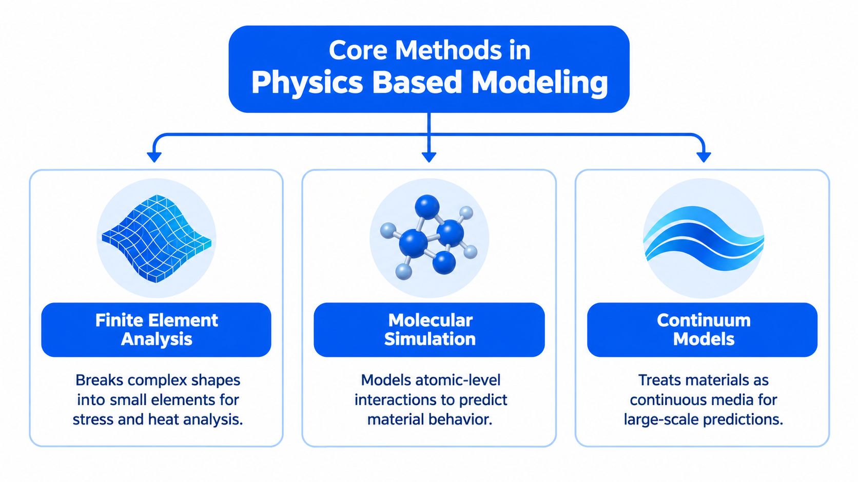
Three families of methods cover most materials problems. They differ mainly in the size of what they describe, and they're strongest when you use them in sequence rather than picking one in isolation.
Finite Element Analysis
Finite element analysis, or FEA, breaks a complex shape into many small elements, like cutting a molded part into a mosaic of tiny tiles. You approximate the governing equations inside each element, then assemble all the pieces into one global system. That lets you predict stress, deformation, and temperature across a real geometry instead of a flat test coupon.
The method has deep roots. Alexander Hrennikoff modeled structural behavior using lattice-like discretization in a 1941 paper, Richard Courant had applied related ideas earlier, and the term finite element method appeared in 1960 in work by John Clough on plane elasticity, as this history of the finite element method describes. By 2021, the method had reached its eightieth anniversary.
The trade-off is direct. A finer mesh gives better spatial resolution but costs more computing time. A coarse mesh runs fast and may miss a stress concentration at a sharp corner. Good modelers refine only where gradients are steep.
Molecular Simulation and Continuum Models
Molecular simulation works at the opposite end of the scale. It follows atoms and polymer chains, so you can see how chains pack, how a filler surface attracts a chain, or how confinement changes mobility. You can't observe those events directly in a lab. Simulation makes them visible.
Continuum models treat material as smooth matter rather than individual molecules. They're appropriate when you care about flow in an extruder, heat conduction in a curing part, or bulk viscoelastic response, and atomic detail would add cost without changing the decision.
Heat flow is a good place to see why scale choice matters. If you're learning why heat treatment matters, a continuum heat equation often explains the temperature profile, while molecular detail helps explain why processing history changed the structure that responds to that temperature.
- Use molecular methods when interfacial adhesion, chain conformation, or local deformation controls performance.
- Use mesoscale or coarse-grained methods when you need larger structures and longer times than atomistic simulation can reach.
- Use FEA and continuum models when geometry, boundary conditions, and nonlinear loading control the outcome.
The mistake to avoid is running the most detailed model by default. Detail you can't calibrate doesn't add confidence. It adds parameters you can't verify.
Physics Based Modeling vs Data-Driven Approaches
A data-driven model and a physics based model answer different questions. A machine learning model asks what pattern links inputs to outputs in the data you've collected. A physics based model asks what mechanism must hold for that link to exist.
Say you're predicting tensile strength from filler loading. A data-driven model can fit your past formulations very well, including interactions you'd never write down by hand. It struggles when you move to a filler it hasn't seen, because it has no concept of stress transfer. A physics based model represents stress transfer explicitly, so it degrades more gracefully outside your data, but only if your equations and parameters describe the new filler.
Side by Side Comparison
| Dimension | Physics-Based Modeling | Data-Driven ML |
|---|---|---|
| Data needs | Needs measured material parameters and boundary conditions | Needs many labeled examples across the range of interest |
| Interpretability | Parameters map to physical quantities you can check | Importances suggest correlations, not mechanisms |
| Extrapolation | Stronger when governing laws still apply | Weak outside the training range |
| Computational cost | High per simulation, especially with fine meshes | Fast to query after training, training can be costly |
| Unknown mechanisms | Fails when the controlling physics is missing | Can capture effects you don't yet understand |
| Failure mode | Confidently wrong if assumptions are wrong | Confidently wrong if new data differs from old data |
Practical rule: Choose physics when the mechanism is known and you need to move beyond your data. Choose data-driven methods when data are plentiful and the mechanism is murky.
Cost comparisons also mislead people. A physics simulation looks expensive because one run takes time. A data-driven model looks cheap because predictions are instant. But generating clean, consistent experimental data to train it may cost far more than the simulation you avoided. Count the full workflow, including experiments, data cleaning, and revalidation when a supplier or process changes.
A Simple Selection Test
Ask three questions before you commit. First, do you know the controlling mechanism well enough to write equations for it? Second, will you need predictions outside your current formulation or process window? Third, can you measure the parameters the model needs with tests you already trust?
If you answered yes to all three, physics deserves the lead role. If you answered no to the first but you have rich historical data, start data-driven and use it to find patterns worth explaining. Most mature teams end up between the extremes, which leads naturally to hybrid approaches.
Hybrid Modeling Strategies
Hybrid modeling combines both instincts. You keep the equations for what you know, and you let data correct or accelerate the parts you don't. The most discussed version is the physics-informed neural network, or PINN.
The diagram below shows the core idea, a bridge between governing equations and a learning system.
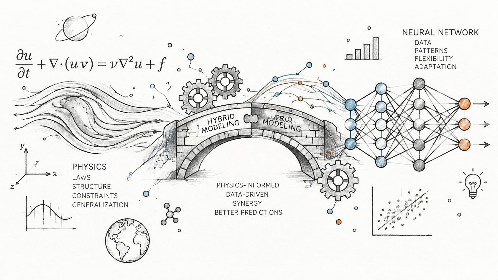
A normal neural network is penalized only when its prediction misses measured data. A PINN is also penalized when its prediction violates a governing equation. In polymer work, that constraint might be a conservation law, a transport equation, reaction kinetics, or a constitutive relation.
What the Polymer Results Actually Show
The reported gains are real but specific. In one ionic-polymer-metal-composite study, a KAN-PINN improved prediction accuracy by 27.54% relative to an MLP-PINN, with average relative errors of 0.316% and 0.277% for two material systems. Another polymerization application reported an 18% reduction in mean absolute error versus a conventional neural network. Both findings come from this review of physics-informed networks in polymer modeling.
The same review reports errors up to 5.26% for difficult deformation states, and notes that extrapolation and noise sensitivity can limit generalization. That's not a reason to dismiss PINNs. It's a reason to stop treating any single headline number as a promise for your system.
This video walks through the hybrid concept visually before you consider deployment details.
In practice, hybrids are most defensible for inverse identification, where you infer a hard-to-measure parameter from easy measurements, for surrogate modeling that speeds up a trusted solver, and for prioritizing the next experiment. They're least defensible as an unvalidated replacement for a mechanistic solver, especially where discontinuities, phase changes, or poorly identified parameters dominate. Keep conventional solvers for those regimes, enforce physics during training where it is reliable, and test on held-out formulations.
Applications in Polymer and Materials R&D
Take a filled polymer composite that keeps cracking near an insert. A single model can't explain it. The crack starts at component scale, but its cause may sit at the filler interface, several orders of magnitude smaller.
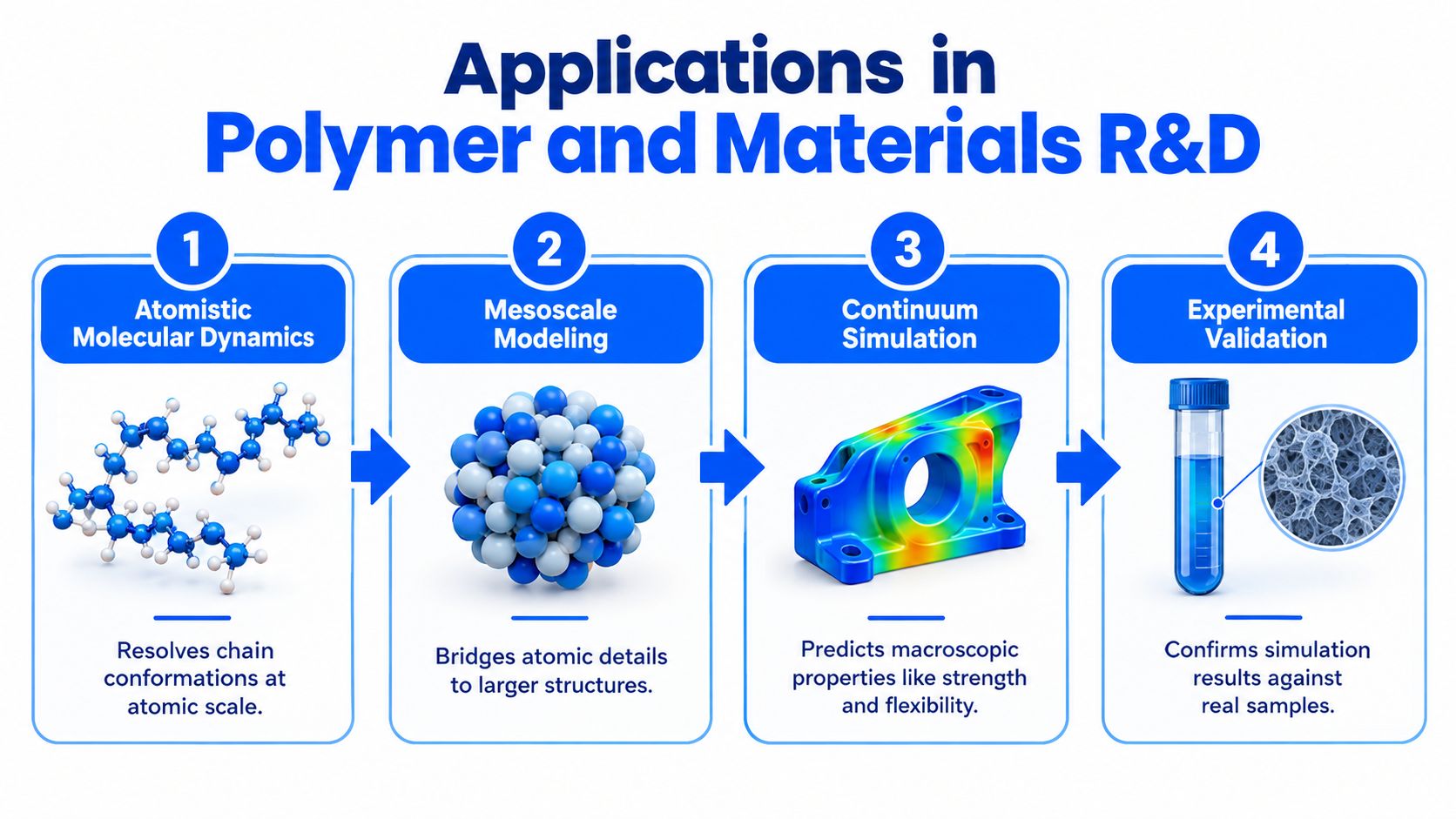
That's why polymer teams use a multiscale workflow rather than one algorithm, an approach detailed in this overview of molecular dynamics and finite element modeling for polymers. Atomistic molecular dynamics resolves chain conformations, interfacial adhesion, confinement, adsorption, and local deformation. Coarse-grained and mesoscale methods extend the length and time scales you can reach. Finite element modeling then maps effective behavior onto engineering geometries, boundary conditions, and nonlinear loading.
Following the Cause and Effect Chain
The logic runs in one direction. Molecular interactions determine morphology and local stress transfer. Morphology controls effective elastic or viscoelastic properties. Those properties determine component deformation, damage initiation, and failure.
An everyday analogy helps. In textiles, structure at the yarn level controls drape and strength at the garment level, which is why a guide to fabric structure for sewists spends so much time on weave before discussing finished fabric behavior. Polymers work the same way. You can't predict part behavior reliably if you've guessed the structure underneath it.
- Atomistic scale: Test whether a coupling agent improves polymer and reinforcement interaction.
- Mesoscale: Examine how dispersion and morphology develop across a larger region.
- Continuum scale: Predict where a molded part deforms or fails under real loading.
- Validation scale: Compare every prediction with a measurement you can repeat.
Calibrate Before You Pass Parameters Upward
The workflow fails when teams pass unchecked numbers between scales. Validate molecular dynamics results on interfacial or cross-linking behavior against spectroscopy, microscopy, or mechanical data first. Then validate the resulting constitutive law against bulk stress and strain and creep measurements.
Finite element modeling is especially valuable for scale-up because it handles complex geometry and nonlinear behavior. It's also the dominant continuum approach for polymer composites. But it is only as reliable as the parameters lower-scale models supply. A beautifully meshed part with a guessed constitutive law gives you precise, wrong answers, which are worse than rough honest ones because they look trustworthy in a review meeting.
Strengths and Limitations of Physics Based Modeling
The strengths are easy to state. Physics based models explain, not just predict. They transfer to new geometries, they expose which parameter controls a result, and they let you run dangerous or expensive conditions virtually. When a model disagrees with an experiment, that disagreement often teaches you something specific about your material.
The limitation people underestimate is simpler. More physics does not automatically mean better predictions.
When Adding Physics Makes Things Worse
If your governing equation is approximate, enforcing it strongly forces the model to repeat your approximation with confidence. Incorrect or poorly calibrated prior knowledge propagates systematic bias. Excessive constraints can also reduce model capacity so much that the model can't fit real experimental behavior, even when the data are trying to tell you something true.
Hybrid models add their own friction. Recent reviews identify recurring problems with non-convex physical loss functions, unstable convergence, sensitivity to the weighting of data and physics terms, and expensive hyperparameter tuning, documented in this assessment of physics-informed modeling trade-offs. Computational cost, inference latency, memory footprint, and implementation overhead are generally not reported, which makes honest comparisons with conventional machine learning difficult.
If a vendor or a paper won't tell you what a model costs to train, tune, and run, you don't have a comparison. You have a demonstration.
Decision Criteria You Can Use in a Review
Judge each proposed constraint on four grounds. Data volume matters because scarce data increases the value of reliable physics. Physics fidelity matters because a well tested law deserves a hard constraint, while a shaky one deserves a soft penalty or none. Computational budget matters because tuning a finicky hybrid can eat the time it was meant to save. Extrapolation risk matters because constraints earn their keep mainly when you leave familiar conditions.
For formulation work, separate two categories clearly. Conservation laws and well characterized transport behavior are reliable across conditions. Mixing history, cure state, morphology, and scale-up effects are empirical process influences that a simplified physical model may not capture at all.
Run ablation studies where you remove one constraint at a time and measure both accuracy and cost. If a constraint doesn't improve held-out predictions, it's decoration, and decoration that slows convergence is a liability your team will pay for on every future run.
Practical Implementation Considerations
A model that matches clean simulation output hasn't proven much. Your real data contain batch variation, instrument noise, missing metadata, process history effects, and inconsistent test protocols. Deployment has to survive that mess, and this discussion of deployment oriented evaluation for physics-informed methods sets out what that requires.
Validate Like an Engineer, Not Like a Benchmark
Report error on held-out experimental data, not only on data the model saw during fitting. Add calibrated prediction intervals so a prediction carries an honest range, and run extrapolation stress tests outside the training domain. A model can satisfy conservation laws and still give poorly calibrated recommendations for a new polymer family, supplier, or production line.
Ask a sharper question than physical consistency. Ask how you'll know when the model is outside its validity envelope, and what experiment you'll run next when it is. If nobody can answer, the model isn't ready to guide spending.
Scale changes need the same skepticism. Moving between atomistic, mesoscale, laboratory, and manufacturing scales isn't automatic, and coarse-grained outputs must be compared carefully against physical properties before you trust them at pilot scale.
A Pre-Deployment Checklist
- Provenance recorded: Who measured each value, on which instrument, under which protocol?
- Failure thresholds defined: At what error or residual level does the team stop and revalidate?
- Domain shift tested: Did performance hold across batches, suppliers, and equipment?
- Prospective validation planned: Will you test predictions on future pilot or production runs before relying on them?
Start narrow. Pick one decision, one mechanism you understand, and one measurement you trust, then expand only after the model predicts something it hadn't seen. Teams that begin with a grand unified simulation usually end with a model no one can validate and no one quite trusts enough to use.
If your team is deciding where physics, data, and targeted experiments should each carry the load, Polymerize can help you unify fragmented experimental data and apply domain-specific, explainable models that predict properties, optimize formulations, and point to the next best experiment with confidence scores. Visit Polymerize to see how materials teams move from trial and error to validated formulations faster, from lab concept through scale-up.
Put your R&D data to work
See how materials teams use Polymerize to plan fewer experiments and reach target properties faster.