
When a viscosity result creeps up for the third batch in a row, do you adjust the formulation, or wait? What if the creep is just the noise you've always had, and adjusting now makes a stable process worse? That question exposes the gap between looking at numbers and judging them. A single result tells you almost nothing about change. A mean control chart gives you a principled way to decide, using your own process history as the reference instead of gut feel or a specification limit that was never designed for that job.
Table of Contents
- What a Mean Control Chart Is and Why It Matters
- The Center Line
- Two Ways to Estimate Variation
- Why Three Sigma
- Steps 1 to 3 Organize and Average
- Steps 4 to 5 Calculate the Limits and Sigma
- Steps 6 to 7 Check the Baseline and Freeze
- The Standard Deviation Version
What a Mean Control Chart Is and Why It Matters
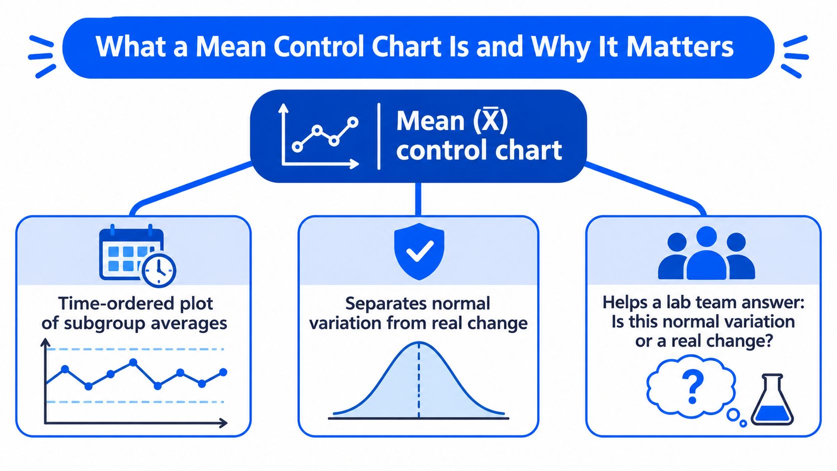
A lab team watching a measured property drift asks one question first. Is this normal variation, or has something really changed? The mean control chart, written as the X-bar chart, answers it by plotting subgroup averages in time order so you can see behavior unfold rather than judge isolated results.
Three elements make up every chart. The plotted points are subgroup means, each one an average of a few measurements taken close together. The center line sits at the grand mean, the average of all those subgroup means. The upper and lower control limits sit three standard errors above and below that line.
Control limits come from your process data. Specification limits come from a customer or design requirement. Confusing the two is the most common first mistake, because a process can be stable and still miss spec, or meet spec while drifting badly.
You'll use this chart wherever you take small groups of repeat measurements. Think viscosity batches, particle size distributions from a dispersion run, cure times, or tensile strength from repeated coupon tests. In each case, you're not asking whether one coupon passed. You're asking whether the average level of the process has moved.
Averaging is what gives the chart its power. Because a subgroup mean varies less than a single reading, the limits narrow by the square root of the subgroup size. Small, sustained shifts that would hide inside individual values become visible against those tighter limits. That's why subgrouping isn't a clerical detail. It's the mechanism that makes the chart sensitive.
What follows builds the skill in order. You'll get the formulas and constants, a worked tensile strength example with real arithmetic, the assumptions that make limits defensible, the signal rules, lab subgrouping choices, and how this chart relates to its companions.
Center Line and Control Limit Formulas
Start with notation, because most confusion here is really notation confusion. Let n be the subgroup size, the number of measurements in each small group. Let k be the number of subgroups in your baseline. For subgroup i, X-bar-i is its mean, R-i is its range (maximum minus minimum), and S-i is its standard deviation.
The Center Line
The center line is always the grand mean, written X-double-bar. You average the subgroup means, so CL = (X-bar-1 + X-bar-2 + ... + X-bar-k) / k. When every subgroup has the same n, that equals the average of all individual measurements. When subgroup sizes differ, each subgroup mean still carries equal weight in this average, which is worth remembering before you defend a limit to a reviewer.
Two Ways to Estimate Variation
The limits need an estimate of short term, within subgroup variation. You can get it from ranges or from standard deviations, and the table below puts both routes in one place so you don't have to hunt across a textbook.
| Element | Range method (R-bar) | Standard deviation method (S-bar) |
|---|---|---|
| Center line | Grand mean X̿ | Grand mean X̿ |
| Upper control limit (UCL) | X̿ + A2 × R̄ | X̿ + A3 × S̄ |
| Lower control limit (LCL) | X̿ − A2 × R̄ | X̿ − A3 × S̄ |
| Within-subgroup sigma estimate | R̄ / d2 | S̄ / c4 |
Here R-bar is the average of the subgroup ranges and S-bar is the average of the subgroup standard deviations. The constants A2 and A3 bundle together the three sigma multiplier, the square root of n, and the correction for estimating sigma from a small sample. That's why the formulas look short. The statistics are hiding inside the constant.
Written out longhand, the standard deviation version is UCL = X̿ + 3S̄ / (c4 × √n), with the matching subtraction for the LCL, where c4 corrects the standard deviation estimate. The range version works the same way once you estimate sigma as R̄ / d2. If you ever need to justify a constant, that longhand form is your justification.
Why Three Sigma
The NIST Engineering Statistics Handbook explains that, under a normal distribution, a point beyond plus or minus three standard deviations has a two-sided probability of approximately 0.0027, or 0.27%, and a one-sided probability of about 0.00135, or 0.135%. With fixed limits, that gives an in-control average run length of roughly 370 plotted samples before a false signal is expected, assuming independent observations and stable conditions.
That rarity is the point. False alarms stay uncommon, so a signal earns investigation. The trade off is that three sigma limits are built to catch substantial shifts, not every small nudge, which is why pattern rules were later added beside them. If you're comparing this logic with automated flagging approaches, the PlotStudio AI guide to anomaly detection is a useful companion on how different methods decide a point is unusual.
Choose the range method for subgroups up to about n = 10, where the range still represents spread well. Choose the standard deviation method for larger subgroups, where using only the maximum and minimum wastes information. Both estimate the same underlying sigma. They differ in efficiency, not intent.
Constants for Subgroup Sizes 2 to 10
The constants d2, c4, A2, and A3 depend only on subgroup size n. They come from the distribution of the range and the standard deviation in samples drawn from a normal population. You never estimate them from your data. You look them up.
Reading the table takes three moves. Find the row for your n. Use A2 with R-bar or A3 with S-bar to set the limits. Use d2 or c4 when you need to convert R-bar or S-bar into a sigma estimate.
| Subgroup size (n) | d2 | c4 | A2 | A3 |
|---|---|---|---|---|
| 2 | 1.128 | 0.7979 | 1.880 | 2.659 |
| 3 | 1.693 | 0.8862 | 1.023 | 1.954 |
| 4 | 2.059 | 0.9213 | 0.729 | 1.628 |
| 5 | 2.326 | 0.9400 | 0.577 | 1.427 |
| 6 | 2.534 | 0.9515 | 0.483 | 1.287 |
| 7 | 2.704 | 0.9594 | 0.419 | 1.182 |
| 8 | 2.847 | 0.9650 | 0.373 | 1.099 |
| 9 | 2.970 | 0.9693 | 0.337 | 1.032 |
| 10 | 3.078 | 0.9727 | 0.308 | 0.975 |
Try two lookups so the habit sticks. For n = 5, A2 = 0.577 and A3 = 1.427. For n = 3, A2 = 1.023 and A3 = 1.954. Notice A2 and A3 shrink as n grows. Larger subgroups give more precise means, so the multiplier needed to reach three standard errors gets smaller.
You can check any A3 value yourself with A3 = 3 / (c4 × √n). For n = 5, that's 3 / (0.9400 × 2.236) = 1.427, matching the table. Running that check once, by hand, does more for your confidence in a review meeting than trusting software output.
Two boundaries matter. n = 1 has no subgroup range, so it uses the individuals chart instead. Subgroups above 10 are uncommon in lab work, so the table stops at 10.
Worked Example of Calculating Limits Step by Step
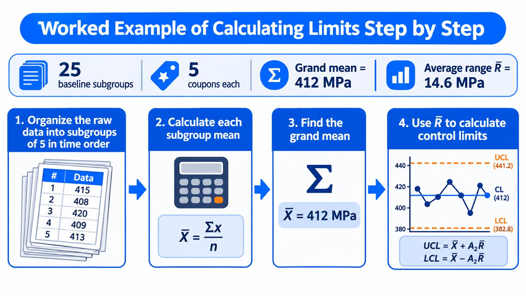
Say you're charting tensile strength from coupon tests during a formulation qualification. You have 25 baseline subgroups of 5 coupons each, taken in production order. Work through the steps in sequence. Each calculation has a reason, and skipping the reason is how limits become indefensible later.
Steps 1 to 3 Organize and Average
Organize the raw data into subgroups of 5 in time order. Keep each subgroup from one batch or one short run, so the five coupons share material, cure conditions, and test setup. Time order isn't optional. Shuffle the rows and you've destroyed the information the chart exists to show.
Compute each subgroup mean and range. For every group of five, average the values for X-bar-i and subtract the minimum from the maximum for R-i. Then average the 25 subgroup means. In this example the grand mean is 412 MPa, and that becomes your center line.
Average the 25 ranges. That gives R-bar = 14.6 MPa. R-bar captures how much coupons disagree within a single short run, before batch to batch differences enter. It's the short term noise floor, and it's what your limits will be built on.
Steps 4 to 5 Calculate the Limits and Sigma
Look up A2 and multiply. For n = 5, A2 = 0.577. So UCL = 412 + 0.577 × 14.6 = 412 + 8.4 = 420.4 MPa, and LCL = 412 − 8.4 = 403.6 MPa. Read that back in plain language. If the process hasn't changed, a fresh subgroup mean should almost always land between about 404 and 420 MPa.
Estimate within subgroup sigma. Divide R-bar by d2 for n = 5, which is 2.326. That gives 14.6 / 2.326 = 6.3 MPa. You don't strictly need sigma to draw the chart, because A2 already contains it. You do need it when someone asks how variable individual coupons are, or when capability questions follow.
Plot the 25 baseline points against the trial limits and look for signals. If a point falls outside and you find a documented cause, such as a misaligned grip on the test frame that morning, remove that subgroup and recalculate. If you find no cause, leave it in. Deleting inconvenient points without a cause gives you limits that are too narrow and a chart that cries wolf.
Freeze the limits and plot new subgroups against them. From here, the numbers 412, 420.4, and 403.6 MPa stay fixed. New batches are judged against that frozen reference. The moment you let software recalculate with every new point, a slow drift gets absorbed into the limits and the alarm never sounds.
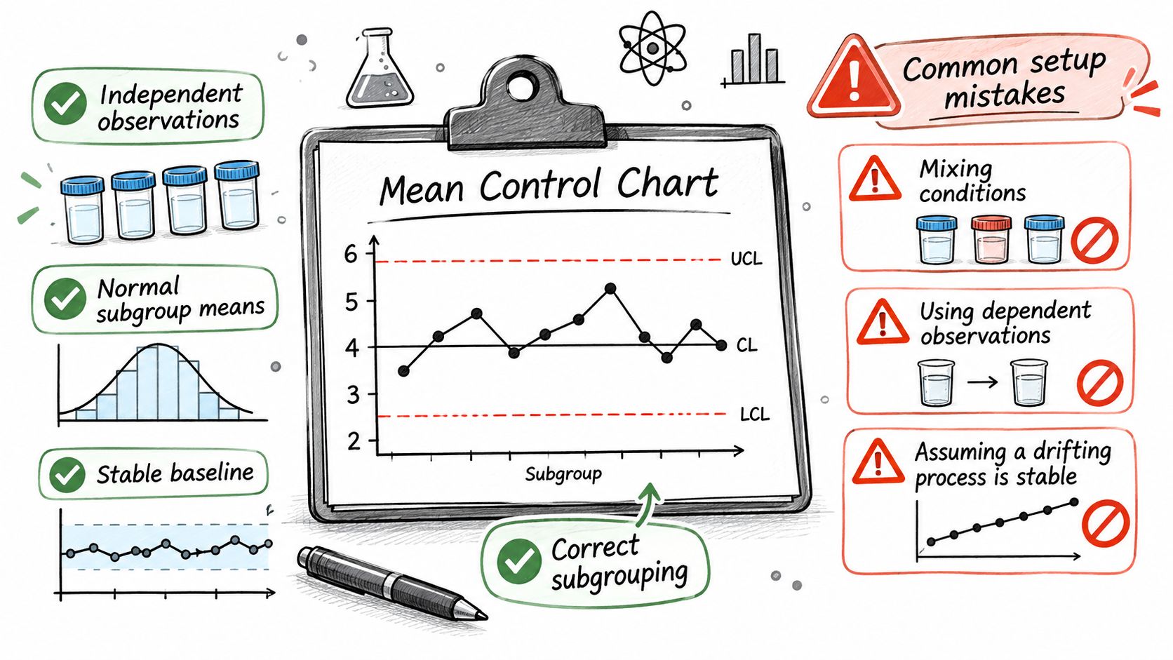
- Independent observations: Measurements within and between subgroups shouldn't be strongly correlated, because correlated points make limits look tighter than they really are.
- Approximately normal subgroup means: Averaging helps here, since means move toward normality even when individual values are skewed.
- A stable process during the baseline: Limits calculated from a process that was changing describe nothing well.
- Rational subgrouping: Each subgroup holds measurements taken under similar conditions, close in time.
Notice what didn't happen. You didn't use the standard deviation of all 125 coupons pooled together. Pooling mixes within run and between run variation, inflates sigma whenever the mean has wandered, and widens the limits until the chart can't see the wandering. Estimating sigma from within subgroup ranges protects you from that trap.
Steps 6 to 7 Check the Baseline and Freeze
Freeze the limits once the baseline is stable. A chart that keeps redefining normal can't tell you when normal has changed.
The Standard Deviation Version
Run the same data through S-bar as a cross check. Suppose the average subgroup standard deviation is S-bar = 6.2 MPa. With A3 = 1.427 for n = 5, UCL = 412 + 1.427 × 6.2 = 420.9 MPa and LCL = 412 − 8.8 = 403.2 MPa.
The two methods land within half a megapascal of each other. That close agreement is expected when the data are stable, because both are estimating the same underlying within subgroup sigma, one from extremes and one from all five values. If your two versions disagree badly, don't average them and move on. Something in your subgroups, often one wild coupon inflating ranges, is worth a closer look. Agreement between methods is quiet evidence your baseline is well behaved, and it's a reassuring line to have ready when a reviewer challenges the limits.
Assumptions and Common Setup Mistakes
The assumption that fails most often in lab data isn't normality. It's rational subgrouping. If one subgroup contains coupons from two batches, or readings from before and after a recalibration, the range inside that subgroup inflates. Your limits widen, real shifts slip through, and the chart looks calm for the wrong reason.
What the Three Sigma Limits Assume
Check each one with a tool you already have. Plot the baseline in time order and look for trends or slow waves that suggest autocorrelation. Put the subgroup means on a histogram or normal probability plot. Read the subgroup log for batch changes, operator swaps, and instrument sessions. None of this needs specialist software. It needs the habit of looking before calculating.
Mistakes That Undermine the Chart
Setting limits from specification limits is the classic error. Specs describe what the customer wants. Control limits describe what the process does. Draw specs on the chart if it helps a conversation, but never judge stability against them.
Recalculating after every new point feels diligent and destroys the method. Each recalculation lets a drift redefine normal. Freeze limits after a stable baseline and change them only after a documented, verified process change.
Mixing batches inside subgroups inflates R-bar and widens limits. Fix it at the source by rebuilding subgroups from one batch and one session. Baselining during a known unstable period, such as the week a mixer seal was failing, bakes that failure into your reference. Wait for stable running, or exclude the period with the cause written down.
Using too few subgroups is the quiet one. Below about 20 subgroups, limits are unstable estimates that jump as data arrives. Treat early limits as provisional, extend the baseline to 20 to 25 subgroups, and then freeze. In small batch lab work that takes patience, but a limit you can't defend helps no one.
Reading Out-of-Control Signals and Their Causes
A signal means the pattern is unlikely under common cause variation alone. It calls for investigation, not automatic adjustment. Twisting a process knob in response to a point you haven't understood is exactly the tampering this chart was built to prevent. Confirm first, then act.
| Signal | Rule | What it usually indicates |
|---|---|---|
| Beyond 3-sigma | One point outside the UCL or LCL | Sudden shift, bad measurement or special cause |
| Two of three beyond 2-sigma | 2 of 3 consecutive points beyond 2-sigma on the same side | Moderate shift in the mean |
| Four of five beyond 1-sigma | 4 of 5 consecutive points beyond 1-sigma on the same side | Small sustained shift |
| Eight in a row | 8 consecutive points on one side of the center line | Persistent offset, such as a new operator or material lot |
| Trend | 6 consecutive points steadily rising or falling | Drift, such as tool wear or reagent aging |
Matching Patterns to Lab Causes
A single point beyond three sigma is often embarrassingly mundane. A bad weighing, a mislabeled sample, a coupon loaded off center. Check the measurement before you check the process, because retesting a retained sample costs minutes and reformulating costs weeks.
The two of three and four of five rules watch the zones between the center line and the limits. Points clustering near a limit, without crossing it, suggest the mean has moved partway and settled. In a lab, think of a new reagent lot that's slightly more concentrated, or a bath temperature controller that's holding a degree high.
Eight in a row on one side is the fingerprint of a persistent offset. Nothing dramatic happened on any single day, but the level stepped and stayed. New operator technique, a replacement sensor, a different supplier grade of the same nominal material. This rule catches shifts too small for the three sigma rule to see quickly.
A six point trend points at something gradually wearing or aging. Reagent degradation, instrument drift, a fouling heat exchanger, a blade losing its edge. Trends reward early attention because they announce tomorrow's out of control point today, while you can still schedule the fix.
A Sensible Response Order
Work in a fixed sequence so signals don't trigger improvisation. First, confirm the measurement, including sample identity and instrument status. Second, check the subgroup log for special causes around that time, such as lot changes, maintenance, or a new analyst. Third, decide whether the process itself needs correction, and record what you found either way.
Caution on rule stacking: Every extra rule you switch on raises the false alarm rate, because each one gives chance another way to look suspicious.
Many teams do well with the three sigma rule plus one or two pattern rules matched to their risk. A high consequence property might justify more rules and more false alarms. A routine screening measurement usually doesn't. Choose deliberately, write the choice in your procedure, and don't add rules after the fact to justify reacting to a point you didn't like.
Choosing Between X-bar, R, S and I-MR Charts
The X-bar chart almost never travels alone. It pairs with a dispersion chart that watches spread, because a mean can hold steady while variation doubles. Compare the four options first, then apply the decision in the order you'd face it at the bench.
| Chart | Data type | Subgroup size | Monitors | Use when |
|---|---|---|---|---|
| X̄ and R | Variables | 2 to 10 | Mean and range | Replicate tests of 3 to 5 per run |
| X̄ and S | Variables | 10 or more | Mean and standard deviation | Larger or unequal subgroups |
| I-MR | Variables | 1 | Individual value and moving range | One measurement per batch or run |
| Attribute charts | Counts or proportions | Varies | Defect counts or rates | Pass or fail results |
Start with how the data arrive. If one test yields one value, such as a single pH reading per batch, there's no subgroup to average. Use I-MR, which plots individual values and the moving range between consecutive points.
If you take three to five replicates per run, use X-bar and R. The range is easy to compute and perfectly adequate at that size. If subgroups run larger, or sizes are unequal because a coupon occasionally breaks before testing, use X-bar and S. The standard deviation uses every value and handles size changes more gracefully.
Always read the dispersion chart first. The X-bar limits are calculated from R-bar or S-bar, so if spread is out of control, those limits rest on a sigma estimate you can't trust. Reading the mean chart alone while variation climbs is the common pitfall here. The paired chart would have shown the climb plainly.
For one value per run data, the I-MR limits are UCL = X-bar + 2.66 × MR-bar and LCL = X-bar − 2.66 × MR-bar, where MR-bar is the average moving range of consecutive points. The constant isn't magic. It's 3 / d2 with d2 = 1.128 for two consecutive values, and 3 / 1.128 = 2.66. That's the same d2 sitting in the n = 2 row of the constants table, which is a good reminder that these charts are one family, not separate inventions.
Applying the Chart to Lab and Formulation Data
How should a lab subgroup reflect the way measurements are produced? Group replicate results that share the same batch and instrument session. A measurement taken after a batch boundary, recalibration, or shift change belongs in a new subgroup, even if that makes the sampling plan less tidy.
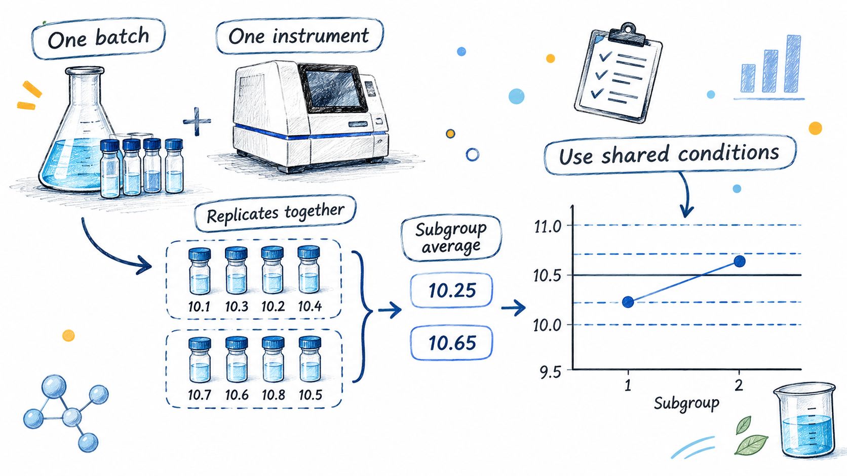
For example, take three viscosity readings from one mixing batch in one session, three particle-size measurements from one dispersion run, or five coupons molded and tested together. Within each subgroup, the range captures short-term variation in measurement and process conditions. Differences between subgroup averages show how the process changes from run to run.
Replicate count affects how much individual noise averages out. With four replicates, the standard error of the mean is half that of a single reading, because √4 = 2. Increasing replicates has diminishing returns: reducing the standard error by half again would require 16 readings. In small-batch labs, consistent subgroup sizes are usually more useful than occasional large ones.
Keep batches separate. If batch-to-batch differences are included in a subgroup range, R-bar rises and the chart's limits widen. That can conceal the formulation shifts the chart is meant to detect. Variation between batches is a signal to examine, not noise to average away.
Record the instrument, operator, reagent lot, and run date beside each subgroup. When a point signals a change, this context helps narrow the search to a relevant event, such as a lot change, rather than leaving analysts to reconstruct the run history.
The video below walks through building and reading a chart. Follow along with recent lab data to see how the subgroup choices affect the plotted averages.
Some experiments produce only one result per run because samples are expensive or the experiment is one-off. In that case, use an I-MR chart rather than forcing replicates. Its limits reflect the greater uncertainty of individual measurements.
Shewhart's chart distinguished routine process variation from variation associated with assignable causes. The 1956 Western Electric Statistical Quality Control Handbook consolidated this approach for separating routine variation from causes that warrant investigation. For lab data, the practical lesson is to treat results as a time-ordered process. A mean control chart can then help identify changes in viscosity, particle size, or cure time before they contribute to a production failure.
Set Up Your First Chart on Real Lab Data
Pick one property with clear customer or process impact, such as viscosity, particle size, cure time, or tensile strength. One chart, run well, teaches your team more than five charts run casually. Resist charting everything at once.
Write your rational subgrouping rule in a log before collecting data, with one batch and one instrument session per subgroup. Then collect 20 to 25 baseline subgroups in time order before calculating any limits. If early points tempt you to compute limits at subgroup eight, remember those limits would be little more than a guess with decimal places.
Calculate the center line and limits using the formulas, constants, and steps you've already worked through. Record every removed point with its documented assignable cause, and remove only points that have one. An unexplained outlier stays, because it says something true about your process.
Once the baseline checks out, freeze the limits and set a fixed review interval, such as weekly. Adjust limits only after a documented process change, never after each new point. Teams that hold this line for one property build exactly the evidence needed to extend charting to others, and to pair it with predictive work. A Japanese TPU manufacturer hit precise targets for 10 material properties across two process flows, with over 95% prediction accuracy, which shows what's possible once process data are trustworthy. Polymerize Labs shows feature attribution maps, causal pathway analysis and confidence scoring, and each prediction comes with contributing factors and similar historical experiments, so a control chart signal can be investigated against the factors that drive the property.
If you're ready to connect disciplined charting with faster formulation decisions, Polymerize unifies your experimental data and layers explainable, property predicting models on top, so drift you detect on a chart can be traced to its drivers and the next experiment planned with confidence. Visit the platform to see how your lab's viscosity, cure, and strength data can start guiding decisions instead of sitting in spreadsheets.
Put your R&D data to work
See how materials teams use Polymerize to plan fewer experiments and reach target properties faster.