

You have years of batch records on one drive, microscope images on another, and a spreadsheet where half the column names changed midway through a project. A formulation worked beautifully in March and failed in June, but nobody recorded what changed. You're supposed to find a stronger, cheaper version without running hundreds more trials.
That's the everyday problem behind machine learning in science. It isn't magic, and it isn't a robot replacing the chemist. It's a disciplined way to learn from past experiments, rank what to try next, and check whether the model deserves your trust before you spend material, time, and budget on its advice.
Table of Contents
What Machine Learning in Science Really Means
Say a materials chemist wants a polymer that's stronger at high temperature. She has formulation ratios, cure conditions, and test results, but no single equation links all of them to strength. An experienced colleague might flip through old notebooks and say, "Batches like this usually fail when the filler climbs too high." A machine learning model does a similar job, only it reads every record systematically and keeps score.
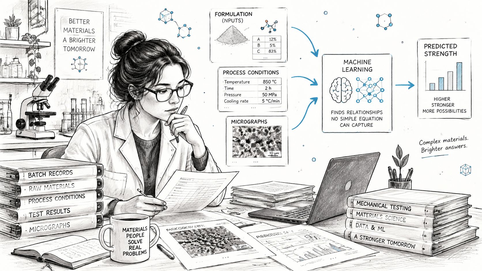
Machine learning means an algorithm learns a mapping from inputs to outcomes from examples, instead of a person writing that mapping by hand. Give it monomer structures and measured glass transition temperatures, and it learns patterns that let it estimate that temperature for a new monomer. Give it prior catalyst screening runs, and it can estimate which untested catalyst deserves a bench slot.
Two Routes to an Answer
A mechanistic model starts from physical law. Quantum chemistry equations, for example, can be precise, but running them across a huge design space is expensive and slow. A data-driven model starts from measured or simulated examples. It answers fast, but it's only reliable inside the range it has already seen. Push it far beyond that range and you're guessing with confidence you haven't earned.
Between them sit physics-informed models. They learn from data while respecting known constraints, such as conservation rules or expected relationships between variables. You get speed without asking the model to rediscover basic physics from scratch.
A useful test: A problem suits machine learning when the outcome is measurable and you have enough past examples, with their conditions recorded, for a pattern to be learned.
Machine learning is a subset of artificial intelligence, but in the lab the goal is usually narrower than the hype suggests. You want a prediction with an error bar, or a ranked shortlist a scientist can test. AlphaFold predicting protein structures from amino acid sequences is the famous version of that idea. Your version might be smaller, but the logic is identical. Learn from examples, predict for new cases, then verify.
Where Machine Learning Fits in the Research Workflow
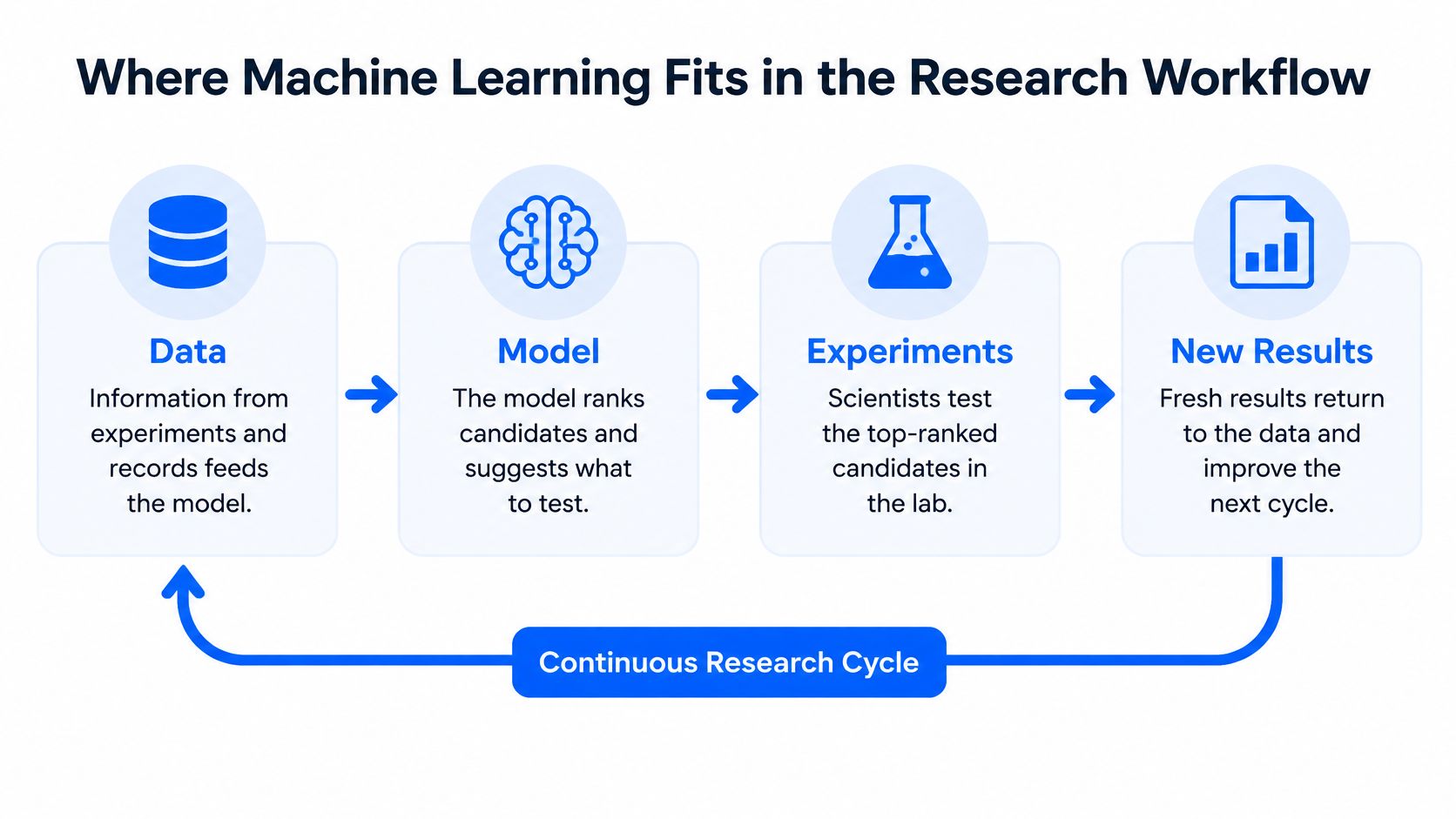
The research loop is simple to state. Data feeds a model, the model ranks candidates, experiments test the top ones, and the new results return to the data. Each cycle should make the next ranking sharper than the last.
The diagram below shows that loop as a continuous cycle rather than a one-off analysis.
| Research stage | ML task | Typical data | Output |
|---|---|---|---|
| Literature and record mining | Text and entity extraction | Papers, patents, lab notebooks | Structured property database |
| Property prediction | Regression and classification | Compositions, process settings, measured properties | Predicted values with error bars |
| Candidate screening | Ranking | Thousands of virtual candidates | Shortlist for physical testing |
| Experiment design | Bayesian optimization and active learning | Past results and budget constraints | Next experiments to run |
| Image and spectra analysis | Computer vision and spectral models | Micrographs, X-ray diffraction, NMR spectra | Quantified structure features |
| Scale-up and quality control | Anomaly detection and process models | Sensor logs, batch records | Early warning of process drift |
Notice how the stages connect. Record mining creates the structured database that property prediction needs. Screening turns those predictions into a shortlist, and experiment design decides which shortlisted candidate you can afford to test first. Image analysis feeds back quantified features, such as particle dispersion, that become new inputs for the next round.
The video below walks through how that cycle looks when scientists run it as a routine, not a special project.
Where's the biggest payoff? Usually it's the stage where experiments cost the most, because every avoided failed run saves material, instrument time, and a scientist's week. Map your own project onto the table and look for the stage where usable data already exists. That's your entry point, even if another stage looks more exciting.
Model Types Scientists Choose and When
Start with the decision, not the algorithm. Are you asking for a number, a category, or the best next experiment? Those are different jobs, and confusing them is how teams buy impressive software that answers the wrong question.
| Model family | Learns from | Strong when | Main limit |
|---|---|---|---|
| Linear and ridge regression | Small descriptor tables | Data is scarce and relationships are near-linear | Misses nonlinear interactions |
| Random forest and gradient boosting | Tabular formulation and process data | Hundreds to tens of thousands of rows | Weak extrapolation beyond the training range |
| Gaussian process regression | Small datasets with uncertainty needs | Tens to hundreds of experiments with calibrated error bars | Computational cost grows with dataset size |
| Neural networks | Large, rich data such as images, spectra or molecular graphs | Large datasets with complex structure | Needs much data and is hard to interpret |
| Bayesian optimization | Results of past experiments | Choosing the next experiment under a fixed budget | Depends on a well-calibrated surrogate model |
| Classification models | Labeled outcomes such as pass or fail | Go or no-go decisions at a candidate stage | Labels are often costly to obtain |
Matching the Model to Your Data
Linear and ridge regression suit small descriptor tables where relationships are close to linear and you need to explain the result to a colleague. If doubling an additive roughly doubles its effect across your range, start here. You'll see quickly whether a simple relationship carries the signal.
Random forests and gradient boosting handle messy tabular formulation and process data well. They cope with interactions you'd struggle to specify by hand, such as an additive that helps only at low temperature. Their weakness is quiet but serious. They interpolate confidently and extrapolate poorly, so a candidate far outside your training range can receive a reassuring score it hasn't earned.
Gaussian process regression is the workhorse for small experimental datasets. Its real value isn't just the prediction, it's the calibrated uncertainty that comes with it. When each experiment costs real money, knowing where the model is unsure tells you where a new measurement buys the most information.
Neural networks earn their place when the data can't be flattened into a tidy table. Micrographs, spectra, and molecular graphs carry structure that these models can read directly. The trade is steep. They need large datasets, careful tuning, and extra work before anyone can say why a prediction came out as it did.
Predictors Are Not Search Strategies
Here's the distinction that trips up many teams. A predictive model estimates a property. A search algorithm decides where to look next. Bayesian optimization belongs in the second camp. It uses a surrogate predictive model, often a Gaussian process, to balance exploiting promising regions against exploring uncertain ones, then nominates the next experiment.
Start with the simplest model that answers the question, and move up in complexity only when validation shows the simple one is failing.
Once a model moves from a notebook into routine team use, versioning, monitoring, and retraining become operational problems, not modelling ones. Data leaders planning that step can use MLOps guidance for enterprise data leaders to think through governance and deployment before the first model reaches production.
Data Needs and Validation Before You Trust a Result
More data isn't automatically better data. Coverage and metadata usually matter more than raw count. A few dozen well-recorded experiments, spread sensibly across your formulation space, can support a Gaussian process model. A neural network trained on thousands of narrow, near-identical examples may still fail on the first new candidate.
Record the context a future model can't guess. Processing conditions, instrument settings, raw material batches, operator, humidity on the day, the supplier lot. Missing context is a common reason predictions fail, because the model attributes an effect to composition when the actual difference was a changed cure schedule nobody wrote down.
What Benchmarks Actually Tell You
Standard benchmarks show how easily a good-looking score can mislead. The Matbench benchmark suite provides 13 standardized supervised-learning tasks spanning 10 datasets, with dataset sizes from 312 to 132,000 samples. Its nested cross-validation protocol is designed to reduce optimistic estimates that creep in when teams repeatedly reuse test data during model selection.
The trap is the random split. If you shuffle your data and hold out a random portion, near-duplicate compositions can land on both sides. The model looks brilliant because it's recognising cousins of examples it already saw, not generalising to new chemistry. Report performance on chemically distinct splits as well, where whole composition or structure families are held out. That number is less flattering and far more honest.
Prospective performance is a sterner test still. In the Matbench Discovery benchmark, universal interatomic potentials achieved F1 scores of approximately 0.57 to 0.82 for stability prediction and discovery acceleration factors of up to 6x within the first 10,000 stable predictions relative to random selection. That framing matters for your lab too. A model earns its keep when its top-ranked candidates succeed, not when its average error looks tidy on a held-out spreadsheet.
Choosing a Validation Method
| Validation method | What it tests | When to use it |
|---|---|---|
| Random train-test split | Average fit on data similar to the training set | Quick first check only, never the final evidence |
| Chemically distinct split | Generalization to new compositions or structure families | Any claim about discovering new materials |
| Prospective experimental test | Whether top-ranked predictions succeed in the lab | Before scaling up or committing a budget |
| Uncertainty calibration check | Whether stated error bars match observed errors | When the model guides which experiment to run next |
| Applicability domain check | Whether a candidate lies inside the range of training data | Before trusting predictions for extrapolated candidates |
Use the table as a matching exercise. If your decision is "which five candidates do we synthesise," then top-ranked yield in a prospective test is your metric. If your decision is "where do we measure next," then check whether the error bars mean what they claim. A model that says it's confident and is routinely wrong will steer your campaign into a ditch.
Before you trust any result, ask three plain questions. Was the test data genuinely different from the training data? Does the candidate sit inside the range the model learned from? Has anyone run the experiment that would prove the prediction wrong? If the answer to any of them is no, you've got a hypothesis. Treat it as one.
Real Use Cases in Materials and Chemistry R&D
AlphaFold shows what happens when the loop works at full scale. The Nature Methods account of the AlphaFold database reports that in the 2020 Critical Assessment of Structure Prediction (CASP) challenge, AlphaFold achieved accuracy comparable to experimental methods for many targets. Its initial public database in July 2021 contained approximately 350,000 predicted structures, including nearly the entire human proteome of about 20,000 proteins, covering 98.5% of the human proteome. One year later it had grown more than 200-fold, to over 200 million predicted structures covering proteins from about 1 million species.
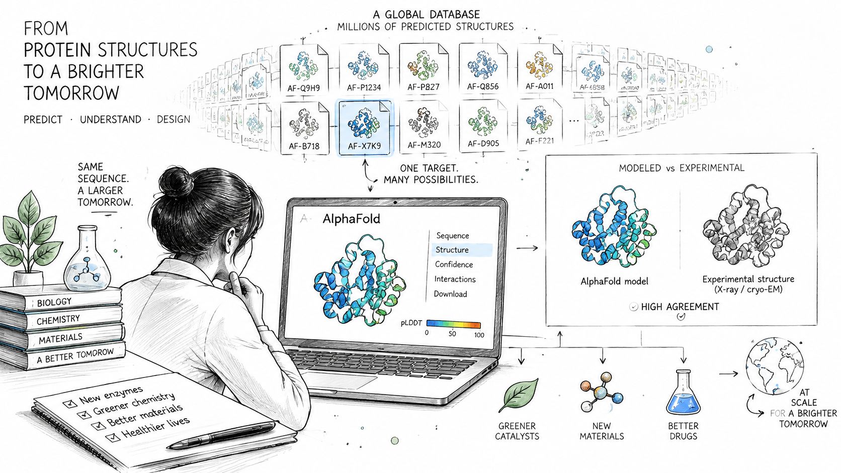
That turned months of laboratory characterisation per protein into immediate computational hypotheses. Experiments didn't disappear. They moved downstream, toward validating and using the predictions. Keep that pattern in mind as you read the smaller cases below.
Polymer Property Prediction
A formulation team links monomer structure and ingredient ratios to properties such as adhesion or conductivity. The model screens combinations the team could never mix by hand, and chemists test only the top-ranked few. The data is historical formulation records, the model is usually a tree ensemble or Gaussian process, and the result is a shorter, better-targeted bench campaign.
Image Analysis of Microstructure
Electron microscope images often get judged by eye. One scientist calls a dispersion "good," another calls the same image "patchy," and neither judgement can be fed into a model. Computer vision converts those images into quantified features, such as particle size distributions and dispersion measures. Once microstructure is a number, you can link it to mechanical performance and find out whether dispersion was driving your failures all along.
Guided Campaigns and Scale-Up
In an active formulation campaign, Bayesian optimization reads the results so far and nominates the next run, steering the search toward better candidates in fewer experiments. During scale-up, anomaly detection models watch sensor logs and batch records for drift, flagging a process that's wandering before it produces a failed production batch.
Every case shares the same skeleton. A structured data source, a model matched to that data, and experiments that check the top predictions. Remove any one of the three and the story falls apart.
Limits, Pitfalls and When Explanations Mislead
An explanation is not a cause. That's the assumption worth challenging first, because it's the one that transforms a useful model into an expensive mistake.
The honest ledger looks like this. On the benefit side, you get faster screening, fewer failed runs, and quantified image features where you once had opinions. On the limit side, everything depends on your data coverage, extrapolation stays weak, and proxy variables can dress themselves up as causes.
Models learn correlations in the data they were given, and scientific datasets are often noisy, incomplete, and biased toward whatever was easy to measure. Watch for these recurring pitfalls.
- Extrapolating beyond the training range: The model has no evidence out there, however smooth its output looks.
- Trusting random-split accuracy: Near-duplicates on both sides inflate the score.
- Ignoring hidden drivers: Batch, supplier, instrument, or laboratory effects can masquerade as formulation effects.
- Treating a high score as discovery: A ranking is a nomination for testing, not a finding.
A feature-importance plot shows what the model used. It doesn't show what caused the result. As a Nature review of explainable machine learning in science notes, an apparent formulation driver may be a proxy for batch, supplier, laboratory, or process conditions, and adding an explanation to a prediction doesn't by itself make that explanation scientifically valid.
So test the claimed driver directly. Change that one variable in a controlled experiment while holding the rest steady. Check the model on out-of-domain samples. Ask what alternative explanation would produce the same pattern, then design the run that separates them. Closed-loop experiments, where each output gets tested and fed back, are the strongest check you have.
Other high-stakes fields have learned the same lesson about acting on model output without verification, and work on safer adoption of healthcare AI makes a useful parallel for any team setting guardrails. A model strengthens a hypothesis. The experiment confirms it.
Choosing Your First Machine Learning Project
Generating hypotheses is now the easy part. Verifying them end to end is the bottleneck, and many teams have no measurable process for it. A 2025 analysis of AI-scientist systems covering 28 papers and five leading AI-scientist systems identified reliable execution and verification, not idea generation, as the central bottleneck. Design your first project around that reality.
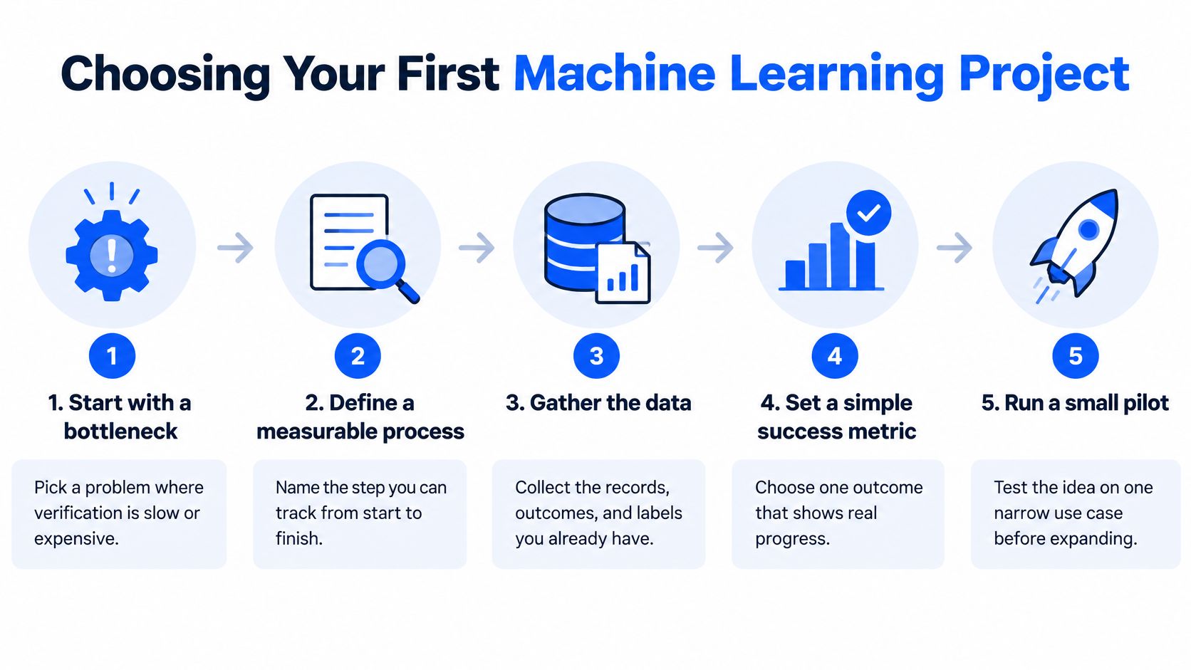
A First-Project Checklist
- Choose one property tied to a decision: Pick something that triggers a go or no-go call on a candidate, not a property that's merely interesting.
- Audit your records for missing metadata: Processing conditions, instrument settings, and batch identity are the usual gaps, and they're cheaper to fix now than after modelling.
- Pick a validation method that matches the decision: Use the validation table logic. Discovery claims need chemically distinct splits and prospective tests.
- Budget for confirmation experiments before training anything: If there's no money to test predictions, there's no project, only a dashboard.
- Agree success metrics in advance: Calibration of uncertainty, replication rate, failed-experiment reduction, and transfer from lab to production beat a single accuracy number.
If you're evaluating platforms rather than building in-house, apply enterprise criteria early. Where IP or personal data is involved, check vendors against standards such as ISO 27001, SOC 2, and GDPR, and ask for evidence on your own data instead of accepting reported gains. Polymerize, for example, unifies experimental records from spreadsheets and electronic lab notebooks and applies domain-specific predictive models to formulation data. Judge it, and every alternative, by the same prospective test you'd apply to your own model.
This week: Pick one project and write down, in one paragraph, what success looks like and which experiment would prove the model wrong. Do that before anyone trains anything.
If your team's records are scattered across spreadsheets, notebooks, and instruments, Polymerize can unify that experimental data into a secure, AI-ready backbone and apply explainable, domain-specific models to predict properties and plan your next best experiment. Visit the site to see how the platform supports verification-driven materials R&D, from first formulation to validated scale-up.
Put your R&D data to work
See how materials teams use Polymerize to plan fewer experiments and reach target properties faster.