


The most popular advice about advanced modelling techniques is also the least useful for formulation teams: choose the model with the lowest validation error. That metric matters, but it doesn't answer the question that determines whether a development program succeeds. Which experiment should the lab run next, and how confident should the team be before moving toward scale-up?
A model can fit historical measurements closely and still fail when a formulation changes polymer grade, molecular weight, temperature, shear rate, or processing route. In industrial materials development, the cost of a wrong decision isn't captured by RMSE. It appears as a failed pilot, an unsafe process window, or a promising formulation that can't be reproduced outside the original laboratory conditions.
The practical role of AI is therefore shifting. Instead of asking a model only to predict a property, R&D teams can use it to rank experiments, expose uncertainty, identify the limits of the training data, and preserve physical constraints. The strongest advanced modelling techniques are the ones that improve the next decision, not merely the next score on a static test set.
Table of Contents
Moving Beyond Static Prediction in Formulation
A formulation model that predicts tensile strength, viscosity, cure time, or thermal behavior from a fixed dataset can be useful. It can also create false confidence. Average accuracy hides the cases that matter most, particularly formulations near a specification boundary or compositions that sit outside the chemistry represented in the training data.
The better question is not, “How accurate is the model overall?” It is, “How does the model behave when the team must choose between several expensive experiments?” That shift changes the design of the entire workflow. A useful system should identify promising candidates, show where predictions are uncertain, and recommend trials that either improve the formulation or teach the model something important.
Why benchmark accuracy has limits
Static validation treats every prediction as if it has equal value. A small error on an easy, well-known formulation can count as much as a large error on a novel candidate that determines whether a scale-up proceeds. R&D decisions don't work that way. The lab needs a ranking of options, a defensible risk estimate, and a way to decide whether an uncertain candidate deserves experimental attention.
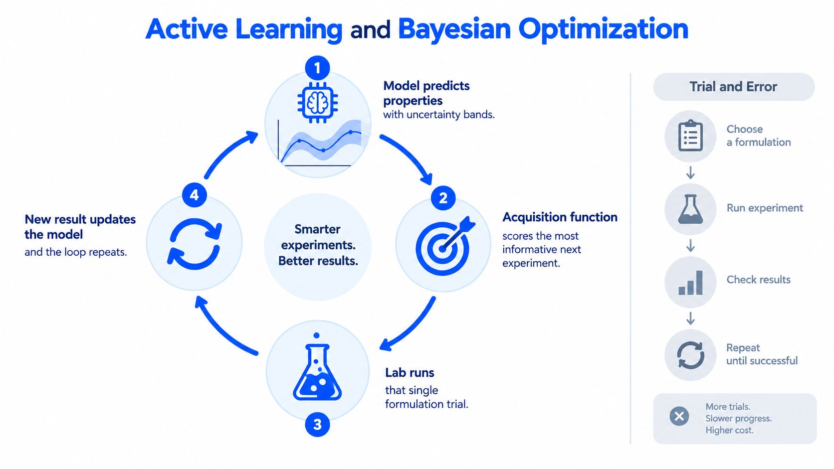
Active learning and Bayesian optimization become more valuable than a marginal improvement in average regression performance. They turn the model into a participant in an experimental loop. The model proposes a candidate, the laboratory generates a result, and that result changes the next recommendation.
Practical rule: Treat uncertainty as an experimental resource. If the model can't explain where it may fail, it isn't ready to guide scale-up.
The same principle applies in adjacent industrial applications. Teams evaluating ML models for predictive maintenance also need to distinguish a reliable signal from an unfamiliar operating condition. In materials R&D, the equivalent is recognizing when a formulation or process state falls outside validated chemical and manufacturing space.
What decision-centric modelling changes
A decision-centric workflow gives scientists more than a predicted value. It provides:
- A ranked shortlist of candidate formulations that meet the desired property profile.
- An uncertainty estimate that distinguishes familiar predictions from extrapolations.
- An acquisition strategy for selecting the next experiment.
- A validation rule that determines whether a prediction is safe enough to influence process decisions.
- A feedback path that sends every new measurement back into the model.
This approach doesn't make experimentation disappear. It makes each experiment carry more information. For formulation teams, that distinction is the difference between automating guesses and building a disciplined search through a difficult design space.
The Evolution of Materials Representation
Before a model can optimize a formulation, it needs a representation that preserves what makes one material different from another. Early materials machine learning often depended on manually designed descriptors, aggregate composition variables, and conventional algorithms such as random forests or support-vector regression. These methods remain useful, especially when datasets are modest and interpretability is essential, but they place a heavy burden on feature engineering.
Graph neural networks changed the modelling question. Instead of describing a material only through a predefined list of features, they can represent atoms, bonds, and crystal structures directly, allowing the model to learn relationships embedded in the material's structure. That matters because materials properties rarely depend on isolated variables. Local bonding, connectivity, symmetry, composition, and structure can interact in ways that a flat feature table may fail to preserve.
A recent review reports that publications applying machine learning to materials research grew by approximately 1.67 times per year over the decade preceding 2023, with more than 2,000 materials-machine-learning papers published in 2023 alone (review of machine learning in materials research). The same review reports a roughly sevenfold reduction in formation-enthalpy prediction error when moving from conventional feature-based methods to graph neural networks on the Matbench benchmark.
Formation enthalpy is important because it provides a core stability-related signal for screening candidate compounds before synthesis or expensive first-principles calculations. The result isn't evidence that graph neural networks automatically outperform every classical method in every industrial dataset. The review also finds that classical machine-learning methods remained dominant overall, which reinforces a more useful conclusion: representation quality must match dataset size, feature quality, interpretability requirements, and validation design.
Choosing the right representation
For polymer and formulation teams, the representation problem looks different from crystalline-material screening. A useful input may need to combine molecular structure, polymer architecture, additives, ratios, processing conditions, batch context, and measurement metadata. A graph representation can capture molecular relationships, but it won't automatically encode mixing history, instrument variation, cure profile, or morphology.
That means teams shouldn't adopt a graph neural network just because it is more advanced. They should first ask whether their data backbone contains the structured inputs such a model requires. If most experiments are stored as inconsistent spreadsheet labels, a complex architecture may amplify data problems rather than solve them.
The same principle applies when materials move from discovery into materials for serial production. A representation that works for candidate screening may need additional process and quality variables before it can support repeatable manufacturing decisions. The model architecture is only one layer. The material representation and experimental traceability determine whether the architecture has anything reliable to learn.
The following video provides additional context on the role of machine learning in materials discovery and modelling:
Active Learning and Bayesian Optimization
Traditional formulation development often runs as a fixed cycle. Scientists select candidates, test them, fit a model, and choose the next batch after reviewing the results. That approach is workable when experiments are inexpensive and the design space is narrow. It becomes a poor use of laboratory capacity when each trial consumes scarce materials, requires substantial preparation, or ends with a destructive measurement.
Active learning changes the question from “Which candidates can we test?” to “Which measurement will improve the next decision?” The model selects an unlabeled candidate for testing, using both expected performance and uncertainty. Bayesian optimization applies this principle when the goal is to find a high-performing formulation with a limited experimental budget.
How the loop works
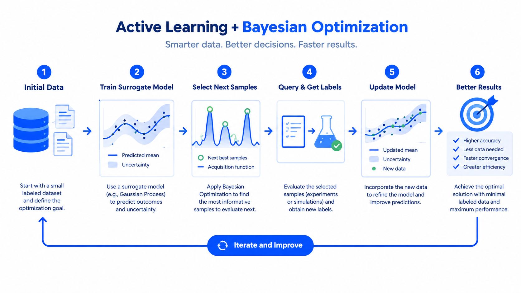
A practical implementation follows six steps:
Train a surrogate model. Use existing experimental results to predict the target property or objective. The model also needs an uncertainty estimate, since a single predicted value cannot show whether a candidate is familiar or speculative.
Define the formulation space. Set chemical, processing, safety, cost, and operational constraints before selecting candidates. A mathematically attractive formulation that cannot be produced consistently should never reach the laboratory queue.
Score candidates with an acquisition function. The acquisition function combines predicted performance with uncertainty. It determines whether the next experiment should test a promising region or examine an unfamiliar one.
Run the selected experiment. Measure the candidate with a documented protocol, then record the formulation, process conditions, batch context, and measurement quality alongside the result.
Update the model. The new observation changes the predicted property surface and the associated uncertainty. That update can alter which formulation appears most useful, even when the measured result is not a new best.
Repeat until the decision threshold is met. Stop when the team has enough evidence to select a formulation, or when further experiments are unlikely to change the decision.
Why Expected Improvement is useful
Selecting only the highest predicted performer exploits the model's current belief. Selecting only the most uncertain candidate explores aggressively, but can spend trials in regions with little formulation value. Bayesian optimization balances both choices.
In a 2022 benchmark of active-learning strategies for materials optimization and discovery, Expected Improvement delivered the best overall performance among the acquisition functions tested (active-learning benchmark for materials optimization). It estimates how much a candidate could improve on the current best result while accounting for uncertainty. A candidate with a slightly lower predicted value can therefore rank highly if its uncertainty creates a credible chance of beating the incumbent.
For polymer development, the objective should reflect how the material will be used, not just its best measured property. A formulation with a high predicted value but a narrow process tolerance may be less useful than one with slightly lower peak performance and a wider operating window. Acquisition functions can target a single property, a multi-property specification, process resilience, or a constrained combination of outcomes.
The same benchmark program's Matbench Discovery evaluation reported discovery-acceleration factors of up to 6 times versus random selection for the first 10,000 stable predictions. It also covered 13 datasets ranging from approximately 300 to approximately 132,000 samples, with F1 scores from 0.57 to 0.82 for leading approaches. These results support model-guided search, but they do not establish a polymer scale-up result. Industrial value comes from choosing experiments that reduce formulation risk and improve the next production decision under actual process constraints.
Quantifying Uncertainty in Polymer Properties
A property prediction without a meaningful confidence estimate is incomplete. In polymer development, the costly error is often false confidence: a model appears certain while predicting a material, processing condition, or property regime that the training data barely represents.
Uncertainty quantification separates familiar interpolation from risky extrapolation. In-distribution uncertainty applies when a candidate resembles known examples. Out-of-distribution uncertainty signals that the model is operating beyond its evidence. That distinction should determine whether a formulation enters a routine test, receives additional characterization, or is held back from scale-up until the evidence improves.
A 2025 benchmark of nine uncertainty-quantification methods across polymer properties found that the strongest method depended on the use case (polymer uncertainty-quantification benchmark). Ensembles performed well on in-distribution data. Bayesian neural networks using Markov-chain Monte Carlo were stronger in difficult out-of-distribution settings, while NGBoost performed particularly well for high-glass-transition polymers.
Matching methods to risk
| Method | Best For | Limitation |
|---|---|---|
| Ensembles | Familiar, in-distribution polymer-property predictions | May be less reliable when candidates are far outside the training domain |
| Bayesian neural networks with Markov-chain Monte Carlo | Challenging out-of-distribution settings | More computationally demanding and operationally complex |
| NGBoost | High-glass-transition polymer use cases | Performance depends on the property and dataset context |
| Novelty and distance checks | Flagging candidates unlike historical data | A distance score alone does not prove that the prediction is accurate |
Choose the method according to the failure mode, not architecture prestige. For chemistry that resembles validated historical formulations, an ensemble may offer a practical uncertainty estimate. A candidate in a difficult extrapolation regime needs stronger scrutiny, and a Bayesian approach may provide better grounds for deciding whether experimental confirmation is justified.
Uncertainty becomes useful only when it changes the experiment queue or the scale-up decision.
Turning uncertainty into an operating rule
R&D leaders can define operating rules such as:
- Low uncertainty and familiar chemistry: allow the candidate into the normal experiment queue.
- Moderate uncertainty near a specification limit: require confirmatory testing before making a process decision.
- High uncertainty or a strong novelty signal: prioritize an informative experiment instead of treating the prediction as a deliverable.
- Uncalibrated uncertainty: stop automated recommendations until the model is recalibrated.
Separate 2025 work on copolymers found that tree-search methods were inefficient for extrapolation, while neural networks and XGBoost improved as training-data volume and range increased. The practical lesson is uncomfortable but important. A more complex model is not automatically safer. Dataset coverage, calibration, novelty detection, and experiment-selection value can matter more than architectural sophistication. For formulation teams, that means uncertainty should guide which experiment happens next, not merely accompany a prediction in a report.
Integrating Physics-Informed Constraints
A model can score well on historical data and still recommend a formulation that violates basic physical expectations. Outside the training range, a surrogate may predict an implausible response to temperature, shear rate, composition, or molecular weight because its loss function contains no constraint against that behavior. For scale-up, that failure matters more than a small improvement in average prediction error.
Physics-informed machine learning addresses the problem by embedding known relationships, conservation rules, monotonicity assumptions, or mechanistic equations into model development. Hybrid workflows combine data-driven surrogates with finite-element, multiphysics, ab initio, molecular-dynamics, or structural-optimization methods. These approaches can narrow the search space and make predictions more defensible, but they also add implementation and validation work.

Data-driven and physics-informed models
A purely data-driven surrogate is usually faster to train and easier to deploy once the data pipeline is stable. It can capture complicated interactions without requiring a complete mechanistic theory. Its limitations become visible with sparse data, noisy measurements, new materials, or a transition from molecular behavior to processing performance.
A physics-informed model constrains the solution space, reducing the chance of implausible extrapolation. Constraints that reflect recognized mechanisms can also make the model easier to interpret. Poorly chosen constraints create a different risk: they can introduce bias, suppress useful discovery, or encode assumptions that apply only within a narrow operating regime.
| Approach | Practical advantage | Operational risk |
|---|---|---|
| Purely data-driven surrogate | Fast iteration and flexible pattern recognition | Can violate physical behavior during extrapolation |
| Physics-informed model | Incorporates known constraints and mechanistic structure | Requires valid physics, careful implementation, and cross-scale testing |
| Hybrid workflow | Uses each method where it is strongest | More integration, calibration, and data-governance work |
The hard test is industrial behavior. A hybrid system must cope with real-world noise, batch effects, instrument variation, semicrystalline behavior, and changing process conditions. Reviews identify uncertainty in noisy environments, extension to semicrystalline systems, and deployment on industrial platforms as unresolved challenges (review of physics-informed and data-driven approaches).
Preserving uncertainty across scales
A molecular prediction does not automatically become a reliable processing recommendation. The workflow should trace measurement error, formulation variability, batch effects, and model approximation through to the final process-window decision. It should also specify recalibration triggers, including a new feedstock source, a changed instrument, or a production condition outside the development dataset.
A 2025 polymer melt-viscosity study tested extrapolation by varying molecular weight, shear rate, or temperature while holding the other variables fixed. It treated a prediction as accurate only when experimental results fell within the predicted uncertainty bounds. That rule tests whether uncertainty is useful under the conditions where the model will be applied, rather than rewarding a low average error on familiar records.
Validation should follow the decision path. If the model will influence processing, test it under unseen processing conditions, not only on randomly held-out formulation records.
A hybrid model earns its place when it helps teams choose safer process windows, reduce failed pilot runs, or identify the measurement most likely to resolve a scale-up risk. Benchmark accuracy remains useful, but uncertainty and physical consistency determine whether a recommendation is safe to act on.
Evaluating Models by Decision Performance
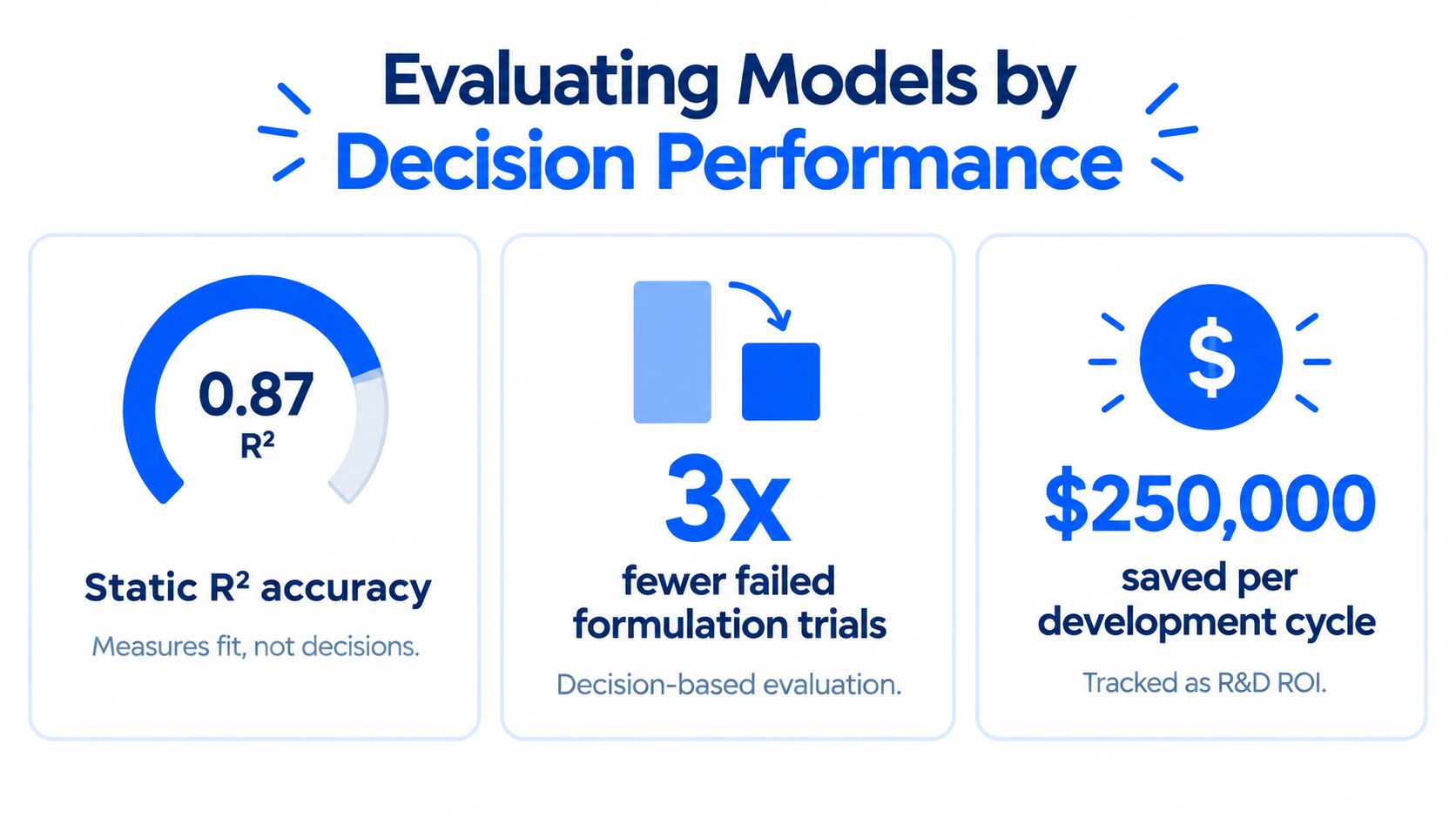
R&D leaders should not treat RMSE and R-squared as complete investment cases. These metrics describe fit on a defined evaluation set. They do not show whether a model selected a useful experiment, detected extrapolation, protected a process window, or helped prevent a failed pilot.
Start evaluation with the decision the model must influence. For formulation recommendations, measure the quality and feasibility of the proposed candidates. For scale-up risk detection, test whether uncertainty identifies difficult conditions. For experiment ranking, determine whether model-selected trials produce more useful evidence than the existing workflow.
A practical evaluation scorecard
Use several layers instead of relying on one headline metric:
- Prediction quality: Break down errors by material family, process regime, property range, and novelty level. An overall average can conceal the subgroup where scale-up risk is concentrated.
- Calibration quality: Check whether predicted uncertainty matches observed outcomes. The polymer melt-viscosity validation rule described earlier links accuracy to uncertainty bounds under the conditions where the model will be used.
- Selection quality: Compare model-selected candidates with those chosen through the current experimental workflow. The relevant measure is how quickly each approach finds useful formulations or informative trials.
- Constraint compliance: Record whether recommendations satisfy chemical, process, safety, equipment, and quality requirements before entering the lab.
- Cross-scale dependability: Test whether a recommendation remains useful after changes in process conditions, batch, instrument, or production environment.
- Operational outcome: Track failed pilot runs, repeat experiments, process-window changes, and time to a validated formulation.
As noted earlier, benchmark programs such as Matbench Discovery report acceleration factors up to 6 times versus random selection. Treat those results as screening context, not evidence that a formulation will survive scale-up.
Making the business case
A model that improves a benchmark without changing laboratory behavior has limited business value. A model with modest static accuracy can still matter if it identifies high-risk extrapolations and helps scientists choose experiments that resolve the next decision.
Agree on the evaluation plan before deployment. Define the target formulation decision, acceptable uncertainty behavior, constraints the model must respect, and production evidence required for sign-off. Then compare model-guided and conventional workflows using the same documentation standard.
Decision performance turns AI from a prediction project into an R&D operating capability. It gives CTOs and VPs of R&D a practical basis for judging whether the system changes development outcomes rather than adding another dashboard. The strongest evidence is a safer process window, fewer failed pilot runs, or a faster path to a formulation that production can reproduce.
Building an AI-Ready Data Backbone
Advanced modelling techniques fail when experimental data lacks context. A property value without its formulation ratio, test method, batch identity, processing history, units, and instrument information may be impossible to interpret later. A centralized data backbone doesn't just make records easier to find. It gives active-learning systems the structured evidence needed to select the next experiment responsibly.
Start with the data that already drives formulation decisions. Don't attempt to standardize every historical record before delivering value. Define a minimum experimental record and enforce it for new work, while progressively cleaning the historical data that supports the first use case.
A practical implementation sequence
Define the decision. Choose one formulation or process decision with a clear experimental loop. Specify the target properties, hard constraints, and uncertainty tolerance.
Create a canonical schema. Standardize material identifiers, composition, units, test methods, process conditions, batch details, instrument metadata, and result quality. Preserve the original value alongside the normalized value so scientists can audit transformations.
Connect existing systems. Bring together spreadsheets, ELNs, laboratory instruments, formulation databases, and production records. Access controls should protect confidential recipes while allowing approved teams to use aggregated evidence.
Record negative results. Failed experiments and rejected formulations define the boundaries of the design space. Excluding them can make a model appear more optimistic than the laboratory experience.
Add uncertainty and provenance. Store replicate variation, measurement error, analyst identity where relevant, and the conditions under which a result was generated. The model needs to know whether two measurements are genuinely comparable.
Introduce active learning carefully. Begin with recommendations reviewed by scientists. Capture why a candidate was accepted, rejected, modified, or delayed, then use those decisions to improve the workflow.
Set recalibration triggers. Define what happens after a feedstock change, instrument replacement, new process regime, or repeated uncertainty failures. A model shouldn't continue operating unchanged when its evidence base has shifted.
Polymerize fits this operating model as one available platform option. Its Polymerize Connect capability unifies experimental data from spreadsheets, ELNs, and other silos into a centralized data backbone, while Polymerize Labs provides domain-specific models for property prediction, formulation optimization, causal drivers, confidence scores, and next-experiment planning. Teams should evaluate it alongside other systems against their own governance, integration, explainability, and prospective-validation requirements.
The final step is adoption. Formulation chemists and process engineers need to see the recommendation, its uncertainty, the relevant historical precedents, and the constraints in the same workflow. If scientists must export data, interpret a disconnected score, and re-enter the result manually, the experimental loop will break even if the underlying model is sound.
Polymerize helps materials R&D teams unify fragmented experimental data, predict material properties, optimize formulations, and plan next experiments with explainable confidence signals. Visit Polymerize to assess how its AI-native platform can support a more disciplined path from formulation discovery to validated scale-up.
Put your R&D data to work
See how materials teams use Polymerize to plan fewer experiments and reach target properties faster.